Tutorials

Gaussian regression

import numpy as np
from vsusp import fit_ridge, s2m

X = np.array([[-2, 0], [-1, 1], [0, -1], [1, 0], [2, 1], [0, -1.]])
y = np.array([-3.8, -2.1, .1, 2.2, 3.9, -.2])
fit = fit_ridge(X, y, draws=200, chains=2, random_state=12)
print(fit.summary())
prediction = fit.predict(X)
path = s2m(fit.pooled_draws(), [.1, .5], feature_names=fit.feature_names)
print(path.summary())

prediction contains posterior means and pointwise equal-tail intervals for the conditional mean. Use include_noise=True, random_state=12 for new-observation intervals. The ridge draws are independent posterior draws. Horseshoe and spike-and-slab fitting use Gibbs sampling instead.

Spike-and-slab draws

from vsusp import fit_spike_slab, spike_slab

fit = fit_spike_slab(X, y, draws=200, burnin=100, chains=2, random_state=12)
selection = spike_slab(fit.pooled_draws(), feature_names=fit.feature_names)
print(selection.summary())

Excluded coefficients are exactly zero. mpm includes variables with inclusion frequency at least 0.5. hppm is the most frequent complete model visited by the draws. It does not certify the most probable model among unvisited models. This short chain illustrates the call; use longer runs and inspect mixing for an analysis. S2M needs zero_draws="empty" to accept entirely zero draws.

Sparse prediction

from vsusp import savs, dss

beta_mean = fit.pooled_draws().mean(axis=0)
print(savs(X, beta_mean).summary())
sparse = dss(X, beta_mean, penalty=.1)
print(sparse.summary())

Use the same column order and units as the supplied coefficients. DSS approximates X @ beta_mean; its approximation error is not held-out predictive error. Check sparse.converged before using it. Neither method selects a penalty by cross-validation or estimates false-discovery rates.

Diagnostics and plots

from vsusp import diagnostics, plot_trace, plot_tuning

print(diagnostics(fit).summary())
plot_trace(fit, variable=0)
plot_tuning(path)

Diagnostics preserve chain identities. Constant variables and single-chain R-hat are reported as unavailable. A good R-hat alone does not establish that a multimodal posterior was fully explored. Plot functions return Matplotlib axes; use ax.figure.savefig("figure.pdf") to save them.

Illustrative figures

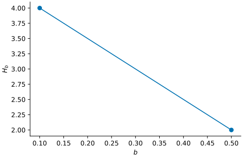
S2M selected counts at two thresholds for the fixed seven-coefficient input.

The tuning path uses the fixed supplied rows, not a simulation study.

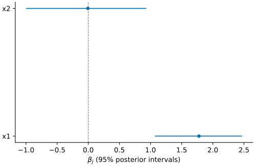
Ridge coefficient means and 95 percent equal-tail posterior intervals for six observations and two predictors.

The ridge illustration has six observations, two predictors and 400 independent posterior draws. Intervals describe this posterior, not selection accuracy.

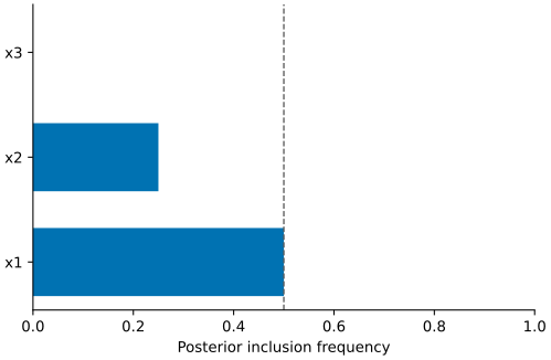
Exact-zero inclusion frequencies for four illustrative coefficient rows, with the MPM cutoff at one half.

These four fixed rows illustrate inclusion counting; they are not fitted data.

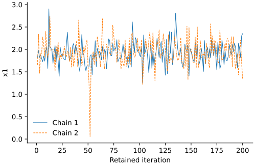
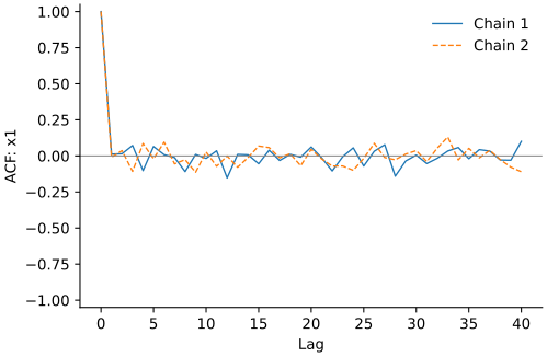
Separate horseshoe traces for the first coefficient across two short chains.

Within-chain sample autocorrelation for the same first coefficient.

The horseshoe illustration uses two chains, 100 burn-in iterations and 200 retained draws per chain, with root seed 12. These short traces illustrate the displays; they do not establish convergence. The figure script and all plotted coefficient draws are provided in examples/figures.py and figures/.