Description

Author: Nilson Chapagain, Texas A&M University.

VsusP selects variables from posterior coefficient draws under Bayesian shrinkage priors. It also fits Gaussian ridge, horseshoe and exact spike-and-slab regression in Python. The runtime dependencies are NumPy and SciPy.

The selection methods follow Li and Pati (2017), with the signal adaptive variable selector (SAVS) and an adaptive-L1 approximation to decoupling shrinkage and selection (DSS) as separate summaries. Model assumptions, tuning and chain mixing determine how fitted results should be interpreted.

Installation

From PyPI:

pip install vsusp

From GitHub:

python -m pip install "git+https://github.com/nilson01/vsusp-python.git"

Or from the package source directory:

python -m pip install .

For figures and chain diagnostics:

pip install "vsusp[plots,diagnostics]"

Worked examples

Gaussian regression

import numpy as np
from vsusp import fit_ridge, s2m

X = np.array([[-2, 0], [-1, 1], [0, -1], [1, 0], [2, 1], [0, -1.]])
y = np.array([-3.8, -2.1, .1, 2.2, 3.9, -.2])
fit = fit_ridge(X, y, draws=200, chains=2, random_state=12)
print(fit.summary())
prediction = fit.predict(X)
path = s2m(fit.pooled_draws(), [.1, .5], feature_names=fit.feature_names)
print(path.summary())

prediction contains posterior means and pointwise equal-tail intervals for the conditional mean. Use include_noise=True, random_state=12 for new-observation intervals. The ridge draws are independent posterior draws. Horseshoe and spike-and-slab fitting use Gibbs sampling instead.

Spike-and-slab draws

from vsusp import fit_spike_slab, spike_slab

fit = fit_spike_slab(X, y, draws=200, burnin=100, chains=2, random_state=12)
selection = spike_slab(fit.pooled_draws(), feature_names=fit.feature_names)
print(selection.summary())

Excluded coefficients are exactly zero. mpm includes variables with inclusion frequency at least 0.5. hppm is the most frequent complete model visited by the draws. It does not certify the most probable model among unvisited models. This short chain illustrates the call; use longer runs and inspect mixing for an analysis. S2M needs zero_draws="empty" to accept entirely zero draws.

Sparse prediction

from vsusp import savs, dss

beta_mean = fit.pooled_draws().mean(axis=0)
print(savs(X, beta_mean).summary())
sparse = dss(X, beta_mean, penalty=.1)
print(sparse.summary())

Use the same column order and units as the supplied coefficients. DSS approximates X @ beta_mean; its approximation error is not held-out predictive error. Check sparse.converged before using it. Neither method selects a penalty by cross-validation or estimates false-discovery rates.

Diagnostics and plots

from vsusp import diagnostics, plot_trace, plot_tuning

print(diagnostics(fit).summary())
plot_trace(fit, variable=0)
plot_tuning(path)

Diagnostics preserve chain identities. Constant variables and single-chain R-hat are reported as unavailable. A good R-hat alone does not establish that a multimodal posterior was fully explored. Plot functions return Matplotlib axes; use ax.figure.savefig("figure.pdf") to save them.

Illustrative figures

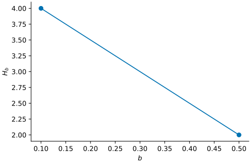
The tuning path uses the fixed supplied rows, not a simulation study.

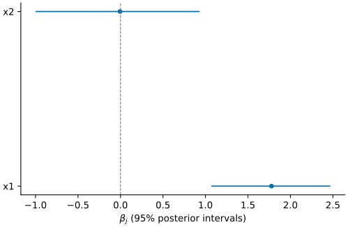
The ridge illustration has six observations, two predictors and 400 independent posterior draws. Intervals describe this posterior, not selection accuracy.

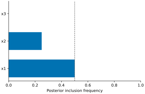
These four fixed rows illustrate inclusion counting; they are not fitted data.

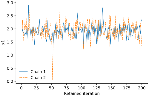
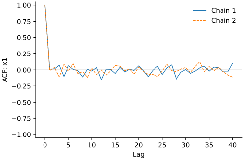
The horseshoe illustration uses two chains, 100 burn-in iterations and 200 retained draws per chain, with root seed 12. These short traces illustrate the displays; they do not establish convergence. The figure script and all plotted coefficient draws are provided in examples/figures.py and figures/.

Methods and limitations

Coefficient-draw selection

Use a finite matrix with draws in rows and coefficients in columns. Remove the intercept. Keep coefficient units unchanged when comparing thresholds.

S2M follows section 2.2.1 of Li and Pati (2017). It recursively splits absolute coefficients and retains the saved lower-mean noise candidate at stopping. Recursion continues while the center gap is greater than b; it stops when the gap is at most b, or a small/constant candidate boundary applies. The signal count is the mode across draws; tied modes favor the smaller count.

Basic 2-M uses the smaller cluster size, which need not be the lower-mean cluster. Both rules rank variables by median absolute coefficient, with larger column indices winning equal-median ties. Sparse spike draws can give zero medians for all variables; a ranking tie can then select a never-included variable. Use inclusion summaries when inclusion probability is the target.

small_set="legacy" retains recursive candidate pairs. "refine" splits a distinct pair. Initial constant magnitudes have no defined split. The explicit all-zero convention assigns zero signals; S2M requires zero_draws="empty". These are boundary choices, not a new selection guarantee. Continuous-prior S2M draws retain at least one signal. No automatic threshold is provided.

Gaussian fitting

The model is

$$ Y = X\beta + \epsilon, \qquad \epsilon \sim N(0,\sigma^2 I). $$

Here Y is the response vector for n observations, X is the model matrix, $\beta$ denotes the coefficient vector and sigma² is the residual variance. The mathematical model includes an intercept; the fitting functions add it internally.

Predictors and response are centered to integrate a flat intercept prior. They are not standardized. The coefficient priors below exclude the intercept, whose prior is flat. The residual variance prior is inverse-gamma with shape 3/2 and scale 3/2. This intercept-prior convention is explicit; the final paper does not supply every fitting detail.

Prior	Coefficient distribution given scales and sigma²
Ridge	$N(0,\sigma^2\mathtt{prior_scale}^2)$
Horseshoe	$N(0,\sigma^2\tau^2\lambda_j^2)$; $\tau,\lambda_j$ independent half-Cauchy(0,1)
Spike-and-slab	Point mass at zero or $N(0,\sigma^2\omega_j^2)$; $\omega_j^2\sim\mathrm{IG}(3/2,3/2)$; inclusion probability $\sim\mathrm{Beta}(1,15)$

The fit stores separate chain and retained-draw axes. draws means retained draws per chain; burnin is additional and is discarded. These differ from the paper's convention of reporting total iterations. Seeds define local NumPy generators and do not modify NumPy's global random state.

A coefficient interval describes the fitted posterior under these assumptions. It is not a repeated-dataset coverage guarantee. These Gaussian fitters do not handle right-censored outcomes as ordinary complete outcomes. Binary, count and survival likelihoods are not implemented.

SAVS and DSS

The signal adaptive variable selector (SAVS) retains coefficient j only when $\lVert X_j\rVert^2|\hat\beta_j|^3>1$, where $X_j$ is predictor column j and $\hat\beta_j$ is its supplied estimate. Equality sets the coefficient to zero. Its threshold depends on predictor units. See Ray and Bhattacharya (2018).

For decoupling shrinkage and selection (DSS), let $\bar\beta$ be the supplied estimate and $\lambda$ the penalty. The sparse coefficient vector minimizes

$$ n^{-1}\lVert X\bar\beta-X\gamma\rVert_2^2 +\lambda\sum_j\frac{|\gamma_j|}{|\bar\beta_j|}. $$

For positive $\lambda$, $\bar\beta_j=0$ constrains $\gamma_j=0$. At $\lambda=0$, the supplied estimate is returned. This is the Hahn–Carvalho adaptive-L1 approximation, not exact minimization of their variable-count penalty. Cyclic coordinate descent reports a relative convex optimality error and warns when the tolerance is unmet. With dependent predictors, sparse coefficients and selected sets may not be unique.

Numerical limits

Fitting stops if a covariance factorization fails or its estimated reciprocal condition number is at most 1e-12. It does not clip prior scales or silently retry a failed chain. Extreme predictor units and prior scales can trigger this limit. Summary and prediction methods reject nonfinite arithmetic; very wide ranges may be unrepresentable in float64. Integer arrays are accepted only when conversion preserves their values.

Function reference

Gaussian models

Here n is the number of observations and p is the number of predictors.

Function	Required inputs	Main controls	Result
fit_ridge	X (n × p), y (n)	draws, chains, prior_scale, random_state, feature_names	GaussianFit
fit_horseshoe	X, y	draws, burnin, chains, random_state, feature_names	GaussianFit
fit_spike_slab	X, y	draws, burnin, chains, random_state, feature_names	GaussianFit

Fitting requires at least two observations, finite numeric inputs and no constant predictor columns. Missing values are rejected. No intercept column should be added. GaussianFit.coefficient_draws has axes (chain, draw, predictor). intercept_draws and sigma2_draws have axes (chain, draw). extra stores prior scales and inclusion states; metadata records seeds and sampling controls.

fit.summary(interval=.95) returns a text table. fit.pooled_draws() explicitly combines chains for selection. fit.predict(X, interval=.95, include_noise=False) returns mean, lower, upper, interval and kind; intervals are pointwise posterior intervals. The point estimate is the posterior conditional mean; observation noise affects the intervals, not that point estimate. Preserve predictor order when predicting.

Posterior selection

Function	Required inputs	Main controls	Result
s2m	draws, thresholds	clustering, small_set, zero_draws, random_state, feature_names	TuningResult
two_means	draws	clustering, random_state, feature_names	SelectionResult
select	draws, count	feature_names	SelectionResult
spike_slab	draws	feature_names	SpikeSlabResult

A draw matrix has axes (draw, predictor). Exclude the intercept. Clustering requires at least two predictors; the other summaries allow one. Exact clustering is the default; clustering="kmeans" uses NumPy Lloyd iterations.

TuningResult contains thresholds, modal counts, per-draw counts, modal frequencies, selected sets and adjacent-set Jaccard similarities. select(i) uses the threshold at zero-based position i. SelectionResult reports selected indices, names, median absolute coefficients and per-draw counts where estimated.

SpikeSlabResult contains inclusion_probability, mpm, hppm, visited_models, model_counts and hppm_ties. Zero means an exact spike; no numerical tolerance converts continuous coefficients to exclusions. Each result has summary().

Sparse coefficients

Function	Required inputs	Controls	Result
savs	X, beta	feature_names	SparseResult
dss	X, beta, penalty	tol, max_iter, feature_names	SparseResult

X must have one nonzero-norm column per beta entry. No centering is added. The result contains coefficients, selected, converged, iterations, objective, diagnostics and metadata. SAVS does not optimize a DSS objective; its objective field is unavailable (NaN). predict(X, intercept=0) returns X times the sparse coefficients plus the supplied intercept. summary() returns a text summary.

Diagnostics and plotting

diagnostics(fit) includes beta, intercept and sigma². For external arrays, use diagnostics(draws, feature_names=...) with explicit (chain, draw, predictor) axes and at least four retained draws. Results contain rank R-hat, bulk/tail ESS, mean MCSE, flags and backend, plus summary(). ESS is effective sample size; MCSE estimates the numerical error of a sampled posterior mean.

Plot	Input	Other controls
plot_tuning	TuningResult	ax
plot_coefficients	GaussianFit	interval, selected, ax
plot_inclusion	SpikeSlabResult	ax
plot_trace	fit or chain array	variable, ax
plot_autocorrelation	fit or chain array	variable, max_lag, ax

All plots return axes. Variable and selected indices are zero-based. Coefficient plots show posterior means and equal-tail intervals, not selection-error rates.

Numerical validation

Fixed calculations

Analytic checks cover exact two-means partitions, S2M stopping, SAVS thresholding, DSS convex optimality, Gaussian conditional draws and the conjugate ridge posterior. Fixed selection and sparse-coefficient results also agree with the repaired installed R VsusP 1.0.0.9000 on R 4.5.0. This reference is not the released CRAN version. Python's default clustering is deterministic; R's is not.

Native posterior checks

Four fixed seven-observation inputs compare Gibbs draws with numerical integration. Horseshoe checks use one predictor with weak or strong fitted signal. Spike-and-slab checks use two orthogonal or correlated predictors. Each uses four chains with 2000 burn-in and 4000 retained draws per chain.

Check	Maximum rank R-hat	Minimum bulk ESS	Minimum tail ESS
Horseshoe, weak signal	1.0017	2415	2560
Horseshoe, strong signal	1.0000	12322	13246
Spike-and-slab, orthogonal	1.0011	2504	2504
Spike-and-slab, correlated	1.0074	413	400

ESS means effective sample size. Compared quantities include coefficient first and second moments, mean residual variance and, for spike-and-slab, inclusion and complete-model probabilities. Quadrature refinements changed the targets by less than 5e-11. Every discrepancy was within the prespecified audit tolerance: the larger of 0.01 and five estimated Monte Carlo standard errors. These broad audit thresholds diagnose large errors; they do not prove exact sampling.

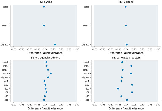
The plotted band is a numerical acceptance rule, not a confidence interval.

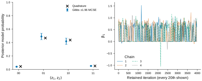
Error bars show ±1.96 estimated Monte Carlo standard errors. Every twentieth retained draw is shown in the traces; all draws enter summaries. The model labels give the two inclusion states. See the numeric results and plot values.

Interpretation

These are low-dimensional posterior checks. They do not establish general selection accuracy, repeated-dataset interval coverage or high-dimensional mixing. The full Li–Pati simulations and lymphoma analysis have not been reproduced. Platform checks are recorded separately from statistical checks.

References and license

Li, H. and Pati, D. (2017). Variable selection using shrinkage priors. Computational Statistics & Data Analysis, 107, 107-119. doi:10.1016/j.csda.2016.10.008.

Ray, P. and Bhattacharya, A. (2018). Signal Adaptive Variable Selector for the Horseshoe Prior. arXiv:1810.09004.

Hahn, P. R. and Carvalho, C. M. (2015). Decoupling Shrinkage and Selection in Bayesian Linear Models: A Posterior Summary Perspective. JASA, 110, 435-448. doi:10.1080/01621459.2014.993077.

Makalic, E. and Schmidt, D. F. (2016). A simple sampler for the horseshoe estimator. IEEE Signal Processing Letters, 23, 179-182. doi:10.1109/LSP.2015.2503725.

Bhattacharya, A., Chakraborty, A. and Mallick, B. K. (2016). Fast sampling with Gaussian scale-mixture priors in high-dimensional regression. arXiv:1506.04778.

Vehtari, A., Gelman, A., Simpson, D., Carpenter, B. and Bürkner, P.-C. (2021). Rank-normalization, folding, and localization: An improved R-hat for assessing convergence of MCMC. doi:10.1214/20-BA1221.

Software and manual: GPL-3.0-or-later. Source attribution is in NOTICE.md.