Continuous outcomes

This small constructed dataset has two exposure scores, x1 and x2, each in 0–3. q=None uses these scores directly. With raw measurements, omit q=None to estimate quartile boundaries from the training data.

import numpy as np
from quantilemix import fit

x1, x2 = np.meshgrid(np.arange(4), np.arange(4))
X = np.column_stack([x1.ravel(), x2.ravel()])
y = 1 + 2*X[:, 0] - 0.5*X[:, 1] + 0.2*(X[:, 0] - 1.5)*(X[:, 1] - 1.5)

result = fit(y, X, q=None)
print(result.summary())
predicted_means = result.predict(X)

Output (joint-effect row from summary()):

Term  Estimate  SE         CI lower  CI upper  t        p-value
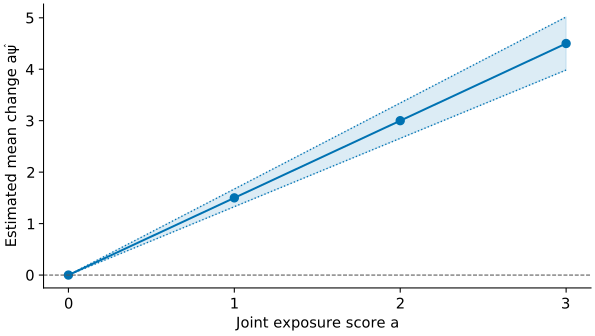
psi   1.5       0.0877058  1.3281    1.6719    17.1026  2.70924e-10

psi = 1.5 is the fitted change in the mean outcome when both exposure scores rise by one. se is the standard error; ci contains normal confidence limits. The p-value uses a separate Student t convention. These illustrative data do not establish coverage or causality.

Download the Python example. For named columns and categorical adjustment, see fit_formula.