QuantileMix reference manual


Version	`0.1.1`
Author	Nilson Chapagain
Contact	`nchapagain@tamu.edu`
Import	`quantilemix`
Requires	Python 3.10 or later; NumPy 2.0 or later; SciPy 1.14 or later
License	GNU General Public License, version 2 or later

Description

Quantile g-computation transforms exposures into ordinal quantile scores and estimates the joint effect of increasing all exposures simultaneously by one quantile. The package supports selected models for continuous, binary, count, and survival outcomes, with more limited support for censored, multicategory, and zero-inflated outcomes. Each API entry documents the effect scale, required inputs, and methodological limitations.

Quantile cutpoints estimated during model fitting are reused for prediction. Sign-specific weights summarize fitted exposure coefficients rather than causal importance. Successful model fitting does not establish the validity of model assumptions or identify a causal effect without additional causal identification assumptions.

The methods follow Keil et al. (2020), https://doi.org/10.1289/EHP5838. Selected results were checked against R qgcomp 2.19.6. This unofficial Python package has not been endorsed by the original authors. Fitting and prediction do not require R.

Citation

Chapagain, N. (2026). QuantileMix: A Python package for quantile g-computation. arXiv:2610.34368.

Record the package version or commit used and cite the statistical method used in the analysis. The citation page provides BibTeX.

Documentation source and adaptations

The reference entries follow the R manual’s Description, Usage, Arguments, Details, Value, Examples and See Also structure. Applicable wording is retained from the GPL-licensed R qgcomp 2.19.6 documentation. Python signatures, containers, restrictions and examples describe this package’s behavior. The adapted source and license are identified in NOTICE.md.

License and credit

Copyright in the adapted R documentation belongs to its original contributors, including Alexander Keil. The Python manual and adaptations are distributed under GPL-2.0-or-later. See LICENSE for the full license terms and warranty disclaimer, and NOTICE.md for attribution. DeepMix is acknowledged as prior partial Python coverage; no DeepMix code was copied.

Using the package

Install and run a Gaussian fit

Install from PyPI:

pip install quantilemix

Or install the latest source from GitHub with Git installed:

python -m pip install "git+https://github.com/nilson01/quantilemix.git@main"

Or, if you have downloaded the source, run this from the folder containing pyproject.toml:

python -m pip install .

In this example, the first two columns are exposure scores and the third column is a continuous outcome:

import numpy as np
from quantilemix import fit

data = np.array([
    [0, 0, 1.0], [0, 1, 0.6],
    [1, 0, 2.1], [1, 1, 1.4],
    [2, 0, 3.0], [2, 1, 2.7],
    [3, 0, 4.2], [3, 1, 3.5],
])
result = fit(data[:, 2], data[:, :2], q=None)
print(result.summary())

Here q=None means the exposure columns already contain scores. Use quantilemix for installation and imports. For a separate Python environment, see the Python Packaging User Guide. Contributor setup and tests are in CONTRIBUTING.md.

Method and interpretation

Keil et al. use \(X_{ji}^{q}\) for the score of exposure \(j\) in person \(i\), \(Y_i\) for the outcome, \(\beta_j\) for an exposure coefficient, and \(\psi\) for the joint effect in their quantile g-computation section. We use those symbols here. We write \(X_i^q\) for the vector of person \(i\)’s exposure scores and \(Z_{i\ell}\) for adjustment covariate \(\ell\), which the paper omits from its displayed additive equation. There are \(n\) observations, \(d\) exposures and \(c\) covariates. The fitted model has \(k=1+d+c\) coefficients and conditional mean

\[ E(Y_i\mid X_i^q,Z_i)=\beta_0+\sum_{j=1}^{d}\beta_j X_{ji}^{q} +\sum_{\ell=1}^{c}\gamma_\ell Z_{i\ell}. \]

The joint effect is \(\psi=\sum_{j=1}^{d}\beta_j\); its estimate is \(\widehat\psi=\sum_{j=1}^{d}\widehat\beta_j\). Holding covariates fixed, the difference between two fitted means whose exposure scores all differ by one is

\[ \widehat m(X_i^q+\mathbf{1},Z_i)-\widehat m(X_i^q,Z_i) =\sum_{j=1}^{d}\widehat\beta_j\{(X_{ji}^{q}+1)-X_{ji}^{q}\} =\sum_{j=1}^{d}\widehat\beta_j=\widehat\psi. \]

Here \(\mathbf{1}\) is a vector of \(d\) ones and \(\widehat m\) is the fitted conditional mean. Both exposure profiles must be meaningful for the intended interpretation. The contrast in \(\widehat\psi\) raises each exposure by one score category, not by one unit of its original measurement. It does not describe an intervention that keeps scores at the top category when they would otherwise rise above it.

In this manual, a hat marks an estimated quantity. Each other method entry defines its own \(\psi\) and states its scale. For example, the Gaussian \(\psi\) is a mean difference, while the additive binary \(\psi\) is a log odds ratio. The two values have different meanings even when the software calls both of them psi. For a common exposure score \(a\), this manual uses \(\widehat\mu(a)\) for a Gaussian standardized mean, \(\widehat R(a)\) for a binary risk, and \(\widehat M(a)\) for a Poisson count mean. Each entry defines its own intervention and adjustment rule. Symbols for methods beyond the paper’s examples are defined in their individual entries.

Confidence interval and p-value for the Gaussian effect

For the variance calculation, let \(\widehat\theta\) collect the fitted intercept, exposure coefficients and covariate coefficients, in that order. This vector notation is only for the calculation; the paper names exposure coefficients separately. The contrast vector \(a\) is zero for the intercept and covariates and one for each exposure. With full design matrix \(D\) and residuals \(e_i\), the ordinary least-squares covariance is

\[ \begin{aligned} \widehat\sigma^2 &= \frac{\sum_{i=1}^{n}e_i^2}{n-k}, & \widehat V &= \widehat\sigma^2(D^{\mathsf T}D)^{-1},\\ \widehat{\mathrm{Var}}(\widehat\psi)&=a^{\mathsf T}\widehat V a =\sum_j\widehat{\mathrm{Var}}(\widehat\beta_j) +2\sum_{j<l}\widehat{\mathrm{Cov}}(\widehat\beta_j,\widehat\beta_l). \end{aligned} \]

The software uses singular-value decomposition, a matrix method, to fit the regression and calculate \(\widehat{\mathrm{Var}}(\widehat\psi)\) without directly forming the inverse shown above. The covariance terms account for the fact that the exposure coefficient estimates can vary together.

The standard error is \(s=\sqrt{\widehat{\mathrm{Var}}(\widehat\psi)}\). For significance level \(\alpha\), R qgcomp 2.19.6’s Gaussian convention uses

\[ \mathrm{CI}=\widehat\psi\ \pm\ z_{1-\alpha/2}s,\qquad p=2\,\Pr\{T_{n-1-d}\geq |\widehat\psi/s|\}. \]

Here \(z_{1-\alpha/2}\) is a standard-normal quantile and \(T_\nu\) has a Student \(t\) distribution with \(\nu\) degrees of freedom. The p-value uses \(n-1-d\), whereas residual variance uses \(n-1-d-c\). Thus the interval and test need not agree at a decision threshold. The interval is not an exact finite-sample \(t\) interval. If the variation is too small to separate from numerical rounding, the software warns that the test result is undefined. The result entry explains this case.

Positive case weights

Case weights give observations different influence in the Gaussian regression. They differ from the descriptive sign weights below. For strictly positive weights \(w_i\), the fitted coefficients minimize \(\sum_i w_i(Y_i-D_i\theta)^2\). Let \(W\) be the diagonal matrix of these weights and \(S\) the weighted residual sum of squares. Then

\[ \widehat\sigma_w^2=\frac{S}{n-k},\qquad \widehat V_w=\widehat\sigma_w^2(D^{\mathsf T}WD)^{-1}. \]

The same joint contrast uses \(a^{\mathsf T}\widehat V_w a\). R qgcomp computes exposure cutpoints before fitting, so case weights do not change them. These model-based limits do not account for complex survey sampling or correlation among observations in the same cluster. The study of 24,000 datasets used equal weights and does not show how often weighted intervals cover the true effect.

For Bernoulli-logit and Poisson-log fits, these are GLM prior weights. Each positive weight multiplies its row’s log likelihood and Fisher information. For integer weights, the coefficients and model-based covariance agree with repeating that row. Formula fits may use missing="drop" to omit rows with missing weights; the returned result saves the retained row positions. Weighted fixed-case agreement does not establish repeated-sample coverage.

Sign weights

Following the paper’s \(w_j\) notation, the fitted sign weight is

\[ \widehat w_j= \begin{cases} \displaystyle\frac{\widehat\beta_j} {\sum_{\ell:\widehat\beta_\ell>0}\widehat\beta_\ell}, & \widehat\beta_j>0,\\[8pt] \displaystyle\frac{|\widehat\beta_j|} {\sum_{\ell:\widehat\beta_\ell<0}|\widehat\beta_\ell|}, & \widehat\beta_j<0. \end{cases} \]

A zero coefficient has no sign weight. The positive weights sum to one, and the negative weights separately sum to one, when those groups are present. They describe the fitted coefficients; no confidence intervals are reported for these weights. Opposite signs can cancel in \(\widehat\psi\) even when individual coefficients are large. Weights are not probabilities of selection or evidence of causal importance.

Example plots: sign weights and fitted means

The two plots use constructed data with three exposure scores. The left plot shows descriptive sign weights. The right plot shows \(\widehat\mu(a)\), the standardized fitted mean when all three exposure scores are set to level \(a\). This example does not show how often confidence intervals cover the true effect across repeated datasets.

Descriptive sign weights

Standardized fitted means

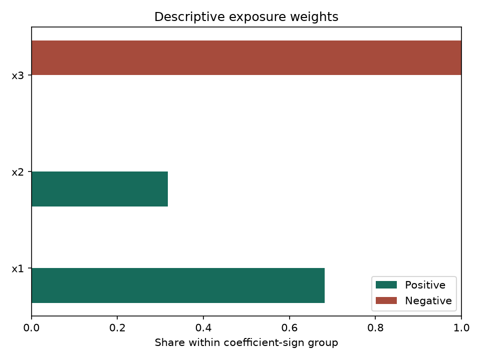
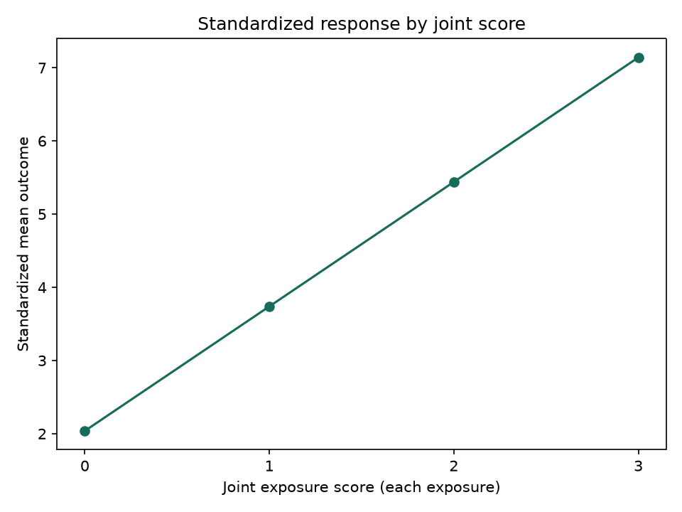
Constructed example. Left: sign weights from a conditional Gaussian fit. x1 and x2 share the positive group; x3 alone fills the negative group. The groups have separate denominators, so their bar lengths do not compare causal importance. Right: standardized means from a separate additive Gaussian row-bootstrap fit. Each point gives \(\widehat\mu(a)\) at the shown score \(a\). The line joins fitted means; it is not an uncertainty band. Twelve seeded resamples make the example repeatable but do not assess interval coverage.

Quadratic Gaussian response to joint exposure changes

The conditional model includes every exposure score and its square:

\[ E(Y_i\mid X_i^q,Z_i)=\beta_0+\sum_{j=1}^d\beta_jX_{ji}^{q} +\sum_{j=1}^d\beta_{j+d}(X_{ji}^{q})^{2} +\gamma^{\mathsf T}Z_i. \]

Set every exposure score to the same level \(a\), retain each row’s adjustment values, and average the fitted means. The paper calls the linear and quadratic mixture coefficients \(\psi_1\) and \(\psi_2\). In the restricted model, \(\widehat\psi_1=\sum_j\widehat\beta_j\) and \(\widehat\psi_2=\sum_j\widehat\beta_{j+d}\). When requested, the model also includes pairwise products \(\beta_{j,k}X_{ji}^qX_{ki}^q\) for \(j<k\), following the paper’s example \(\beta_{1,2}\). Exposure-covariate products are a package extension; we write them as \(\eta_{j\ell}X_{ji}^qZ_{i\ell}\). Then \(\widehat\psi_2\) also includes \(\sum_{j<k}\widehat\beta_{j,k}\), while \(\widehat\psi_1\) also includes \(\sum_{j,\ell}\widehat\eta_{j\ell}\overline Z_\ell\), where \(\overline Z_\ell\) is the sample mean of covariate \(\ell\). Each bootstrap draw uses its own sampled covariate mean. The fitted mean change from \(a\) to \(a+1\) is \(\widehat\psi_1+(2a+1)\widehat\psi_2\), so it depends on the starting level. The API’s effect_at(a) evaluates this change.

Exposure cutpoints are fixed before row-bootstrap resampling. The covariance of the two saved resampled coefficients gives their uncertainty; normal-based confidence limits and Student \(t\) p-values follow the restricted R qgcomp 2.19.6 degree-two convention. Two fixed installed-R comparisons verify the software calculation, not repeated-sample interval coverage. Separate fixed R cases also verify pairwise and exposure-covariate products. This method does not include clusters, case weights or other outcomes.

The separate fit_quadratic_gaussian_ee uses the same intervention curve for repeated observations with known cluster IDs. Its robust covariance sums both conditional and marginal scores within each cluster. Positive case weights enter those scores but leave exposure cuts unweighted. The fitted curve agrees with three fixed installed-R cases. For nonlinear formulas, R qgcomp 2.19.6 forms cluster scores from a saved model frame: after it changes exposure columns, squared and interaction columns can retain their original values. Python rebuilds these terms at each intervention. A separate fresh-design R calculation agrees with Python’s covariance, while the installed R interval can differ. These fixed checks do not establish repeated-dataset interval coverage.

Assumptions and limits

The covariance calculation assumes independent observations and the same conditional error variance for each observation. Exact small-sample calculations also require a correct normal-error model and enough independent model columns to estimate every coefficient. A successful fit does not verify these assumptions. The Gaussian validation study uses known scores from fixed population cutpoints. It does not show how intervals behave when cutpoints are estimated from each dataset.

A causal interpretation additionally needs a well-defined intervention, consistency between observed and intervention outcomes, adequate joint exposure support for the exposure combinations being compared, no effect of one person’s exposure on another person’s outcome, and sufficient control of confounding. These conditions depend on the study design and subject knowledge; software diagnostics cannot establish them. The API entries describe the supported nonlinear, interaction, clustered and resampling methods. The coverage map lists other methods and limits.

API reference

In a Python function signature, an argument without a default is required; one with a default may be omitted. After *, supply arguments by name. The examples show valid calls, not full signatures. Each entry lists its other settings.

Exposure scores and inputs

`quantize`: Assign scores to exposures

Description

Assign each exposure an ordered score. The function can calculate group boundaries from the data, use boundaries you supply, or accept scores you have already assigned. It saves the scores and, when boundaries are used, saves them so new observations can be scored in the same way.

Usage

from quantilemix import quantize

quantization = quantize(exposures)

Arguments

Argument	Meaning and accepted inputs
`exposures`	Nonempty real, finite array of shape `(n, d)`, or a vector for one exposure. No missing or actively masked entries. Labels, when provided, must be unique.
`q`	Default `4`. Requested automatic group count: an integer from 2 to 100,000, excluding booleans. Ties may reduce the fitted count. `None` with no breaks means that inputs are already nonnegative integer-valued scores below \(2^{53}\).
`breaks`	Default `None`. One finite, strictly increasing vector per exposure, including both outer endpoints; lengths may differ. A single vector is accepted for one exposure. Supplied breaks take priority over `q`. This is an alternative to using `q` to define cutpoints.

Details

With automatic grouping, a continuous exposure is represented by scores \(0,\ldots,q-1\), subject to reductions caused by ties. For example, score 1 identifies observations in the second fitted category. These are ordered numeric scores, not a matrix of separate binary indicators.

Automatic mode uses type-7 empirical quantiles, removes duplicate values from the full quantile sequence, and replaces its outer endpoints by \(-10^{64}\) and \(10^{64}\). A value exactly on an interior cut belongs to the lower category. The outer endpoints are included. Automatic training magnitudes must be strictly smaller than \(10^{64}\). Constant exposures are rejected in automatic mode; ties can otherwise reduce the result to one category, which cannot identify a regression coefficient.

Explicit mode keeps the supplied endpoints. Values outside those endpoints raise an error; the endpoints are not automatically expanded. Prequantized mode retains the supplied scores and stores no cutpoints. Scores need not be consecutive. This mode is narrower than R’s general untransformed q=NULL input mode.

The mode field is "quantile", "explicit" or "prequantized". The stored q is the requested integer only in automatic mode. It is None in both other modes, even when a q value was supplied with explicit breaks. The upper bound of 100,000 automatic groups limits allocation in this implementation; it is not a restriction of the statistical method.

Errors.

ValueError is raised for invalid numeric inputs, masks, shapes, labels, group counts or cut vectors; observations outside supplied endpoints; invalid prequantized scores; automatic constant exposures; or automatic training magnitudes at least \(10^{64}\). The function does not fit a model, check regression rank, or emit QGCompWarning.

Value

A QuantizationResult containing read-only scores, saved boundaries, category counts, feature names, training ranges and diagnostics. Its transform method applies the saved map to new observations.

Examples

from quantilemix import quantize

tied = quantize([0, 0, 0, 1], q=4)
print(tied.scores.ravel())       # [0. 0. 0. 1.]
print(tied.category_counts)      # (2,)
print(tied.diagnostics["reduced_category_columns"])  # ('x1',)

explicit = quantize([0, 1, 1.5, 2, 3], breaks=[0, 1.5, 3])
print(explicit.scores.ravel())   # [0. 0. 0. 1. 1.]
print(explicit.mode, explicit.q) # explicit None

In the first example, ties reduce four requested groups to two. In the second, the exact boundary value 1.5 belongs to the lower category.

Source note.

The title, category-score explanation and alternative-cutpoint wording are retained or adapted from Alexander Keil’s R qgcomp 2.19.6 man/quantize.Rd, printed manual pages 76–77, GPL (version 2 or later). The Python array interface, complete boundary vectors, mode restrictions and result object replace the R data-frame and column-selection interface.

`QuantizationResult`: Exposure scores and their saved transformation

Description

The object returned by quantize and either transform method. It stores scores, the original exposure map, and diagnostics for the rows represented by those scores.

Usage

quantization = quantize(exposures, q=4)
quantization.scores
quantization.breaks
quantization.transform(new_exposures)

Arguments

Obtain the object from quantize or transform. The generated dataclass constructor requires internal label state and does not validate manually supplied fields.

Details

Results made by quantize or transform cannot be changed in place: their stored arrays and mappings are read-only. A transformed result retains the original map’s boundaries, training ranges and fitted category counts. Its scores and diagnostics describe the new rows. It does not replace the training map.

The saved category count can differ from the number of categories present in new data. When boundaries are available, the saved count includes categories that no new observation occupies. With previously assigned scores, no full list of possible categories was supplied. The saved count is then the number of distinct training scores, which need not equal the largest score plus one.

Value

Nine public fields are available:

Field	Meaning
`scores`	Read-only float array `(n, d)` or `(m, d)`; integer-valued exposure scores for the represented rows.
`breaks`	Tuple of read-only boundary vectors, including outer endpoints; `None` in prequantized mode.
`category_counts`	Tuple of fitted bin counts, or distinct training score counts when no boundaries were supplied. Preserved by transform.
`mode`	`"quantile"`, `"explicit"` or `"prequantized"`.
`q`	Requested group count in automatic mode; `None` in explicit or prequantized mode.
`feature_names`	Tuple of exposure names in column order.
`training_min`	Read-only vector `(d,)` of minima of the original training inputs, before grouping.
`training_max`	Read-only vector `(d,)` of corresponding training maxima.
`diagnostics`	Read-only mapping with the six keys below.

The public method is transform. There is no summary() method. The underscore-prefixed label field is internal state.

Quantization diagnostics.

All row indices and bin numbers are zero-based. The same mapping appears under result.diagnostics["quantization"] for training observations.

Key	Meaning
`extrapolated_rows`	Tuple of row positions having at least one exposure below its training minimum or above its training maximum.
`extrapolated_columns`	Tuple of names having at least one such observation.
`extrapolated_counts`	One count of such values per exposure.
`observed_category_counts`	One distinct-score count per exposure in the currently represented rows. May differ from saved `category_counts` after transformation.
`empty_bins`	With boundaries, one tuple of currently unoccupied fitted bin numbers per exposure. `None` in prequantized mode because the complete category domain was not specified.
`reduced_category_columns`	Names whose number of fitted bins is less than requested `q`. Only automatic mode can populate it.

Initial training extrapolation counts are zero by construction. Neither these counts nor observed categories establish adequate joint exposure support or validate the regression model.

Examples

from quantilemix import quantize

quantization = quantize([0, 2, 8, 10], q=4)
print(quantization.scores.ravel())   # [0. 1. 2. 3.]
print(quantization.breaks[0])
# [-1.0e+64  1.5e+00  5.0e+00  8.5e+00  1.0e+64]
print(quantization.feature_names)    # ('x1',)
print(quantization.training_min)     # [0.]
print(quantization.training_max)     # [10.]

Source note.

R qgcomp 2.19.6 man/quantize.Rd describes returned quantized data and retained cutpoints. This Python class extends that organization with explicit mode, category-count, training-range and diagnostic fields. It does not reproduce the R list interface.

`QuantizationResult.transform`: Score new data with saved cutpoints

Description

Apply existing category boundaries to new exposures without calculating new cutpoints. In prequantized mode, check and retain the new scores.

Usage

transformed = quantization.transform(exposures)

Arguments

exposures: nonempty real, finite array (m, d), or a vector for one exposure. It must have the fitted column count and order. When the original inputs were labeled, names and order must match exactly, including the presence of labels.

Details

The original boundaries, mode, names, category counts and training ranges stay the same. Diagnostics identify new observations outside the original training ranges. Crossing a training range alone does not trigger a warning.

ValueError is raised for invalid data, shapes, masks or labels; an exposure count different from the fitted map; values outside saved endpoints; or invalid prequantized scores. For automatic maps, new values can enter the extreme bins beyond the training range, provided they lie within the saved \(\pm10^{64}\) endpoints. No regression is fitted.

Value

A new QuantizationResult. Its scores and diagnostics refer to the supplied rows; its map metadata remains unchanged.

Examples

from quantilemix import quantize

quantization = quantize([0, 1, 2, 3], q=2)
new = quantization.transform([1.5, 2])
print(new.scores.ravel())        # [0. 1.]
print(new.category_counts)      # (2,)

The original cut is 1.5. The value equal to that cut belongs to the lower category; cutpoints are not recomputed from the two new observations.

`qgcomp`: Select an additive model from a formula

Usage

from quantilemix import qgcomp
result = qgcomp("y ~ x1 + x2 + z", data, ("x1", "x2"),
                family="gaussian", q=4)
binary_rr = qgcomp("y ~ x1 + x2", data, ("x1", "x2"),
                   family="binomial", B=200, seed=17)
binary_or = qgcomp("y ~ x1 + x2", data, ("x1", "x2"),
                   family="binomial", rr=False, q=2)
survival = qgcomp("Surv(time,event) ~ x1 + x2", data,
                  ("x1", "x2"), family="cox", q=4)

Arguments and routing

formula names an outcome, exposures and adjustment terms; data supplies named columns and exposures lists the exposure names. C(z) encodes a categorical adjustment column, with sorted levels and the first as reference. Gaussian and Poisson outcomes use the existing conditional additive fitters. For a binary outcome, the default rr=True selects a marginal risk ratio with fixed-cut row-bootstrap uncertainty. With the default q=4, its one-category ratio is the exponentiated slope of a degree-one log-risk marginal model. Set rr=False to select the conditional log odds-ratio fit. The ratio and odds ratio are different measures; switching between them changes the scientific question. R ignores rr for Gaussian and Poisson outcomes, and so does this dispatcher. An additive Surv(time,event) formula with family="cox" selects the conditional Cox fit. It accepts complete rows, positive case weights, exact integer cluster IDs and known log-hazard offsets; it does not select a marginal Cox bootstrap.

q, breaks and alpha pass to the selected fitter. weights and missing="drop" are available for the conditional fits. B and seed are available only for the binary risk-ratio route. An exposure_time column name gives a Poisson observation-time offset; its additive route remains conditional, as in R. The Python formula omits the R term offset(log(time)) and instead uses exposure_time="time". An explicit R-style offset term in the Python formula is rejected.

Limits and value

The binary marginal method requires complete numeric data without case weights and may fail on a separated or boundary bootstrap draw. Its four-level interval was assessed in four known-score conditions (4,000 datasets; see the study report). Formulas with nonlinear terms or zero-inflated outcomes, and other unsupported formulas, raise an error. The function returns the unchanged result type of the selected fitter. Six original routes and two four-level binary cases agree with isolated installed R qgcomp 2.19.6. The dispatch and four-level comparison reports give the saved values and limits.

`simdata_quantized`: Generate example data with exposure scores

Usage

sample = simdata_quantized("survival", n=100, coef=[0.2, -0.1],
                           q=4, scale0=5, seed=17)

Arguments and Value

outcometype is "continuous", "logistic", "survival" or "multinomial". coef has one entry per exposure, except multinomial outcomes, where it has one column per nonreference outcome category. corr controls how often later exposures copy the first exposure’s score, or its reverse order for a negative value. It does not set an exact Pearson correlation. n, q, b0, yscale, shape0, scale0 and censtime control sample size, exposure levels and outcome generation. seed uses a local NumPy generator. The read-only QuantizedSimulation mapping contains x1, x2, and an outcome y, or survival time and event indicator d. Its truecoefs property holds known generation coefficients separately. to_dict() returns editable column copies. It can be passed as named data to formula fitters. When ncheck=True, Python increases n to the next multiple of q; R 2.19.6 adds the remainder instead. Python also uses the supplied survival scale0, which that R version does not forward. Identical numeric seeds do not give identical Python and R draws.

`impute_leftcenslognorm`: Left-censored lognormal imputation

Usage

values = impute_leftcenslognorm(y, ry, x, lod=1.0, seed=17)

Arguments and Value

ry marks observed positive values in y; wy defaults to their complement and selects the censored rows to impute. x is a complete numeric predictor matrix without an intercept. lod is a positive scalar or one limit per row; if omitted, the smallest observed value is used. The function fits a lognormal model using observed values and the fact that censored values lie below their limits. It draws model parameters using a normal approximation based on the fitted information matrix, then draws each replacement value below its limit. It returns positive imputed values in selected-row order. impute_tobit is the same function, not another algorithm. This is a Python helper for an external imputation workflow, not an R mice callback or a pooling method. Fixed input checks pass; installed-R agreement and repeated-imputation calibration remain open.

Gaussian models and results

`fit`: Additive Gaussian quantile g-computation

Description

With automatic quantile grouping, the following description from R qgcomp applies:

This function estimates a linear dose-response parameter representing a one quantile increase in a set of exposures of interest. This function is limited to linear and additive effects of individual components of the exposure.

The Python function fits a continuous outcome using an intercept, exposure scores and optional numeric adjustment covariates. It returns \(\widehat\psi=\sum_j\widehat\beta_j\), the sum of fitted exposure coefficients, and its model-based uncertainty. For supplied boundaries or prequantized scores, \(\widehat\psi\) is the fitted mean change when every exposure score increases by one category.

Usage

from quantilemix import fit

result = fit(y, exposures)

Arguments

Let \(n\) be the number of observations, \(d\geq1\) the number of exposures, and \(c\) the number of adjustment covariates.

Argument	Meaning and accepted inputs
`y`	Nonempty real, finite outcome vector of shape `(n,)`. A column matrix of shape `(n, 1)` is rejected.
`exposures`	Real, finite exposure array of shape `(n, d)`. A vector of shape `(n,)` represents one exposure. All selected columns contribute to \(\widehat\psi\).
`covariates`	`None` by default, or a real, finite array of shape `(n, c)`; a vector represents one covariate. These coefficients adjust the model but do not enter the joint sum. For this array entry point, encode categorical covariates in advance; `fit_formula` handles complete text categories. Do not supply an intercept column. Use `None`, rather than an empty-column matrix, when there are no covariates.
`q`	Requested number of quantile groups; default `4`. In automatic mode, an integer from 2 through 100,000; booleans are invalid. With `q=None` and no breaks, inputs must already be nonnegative integer-valued scores strictly below \(2^{53}\). Supplied breaks take priority.
`breaks`	Default `None`. When supplied, use one finite, strictly increasing vector per exposure, including both outer endpoints. Vector lengths may differ across exposures. One vector is sufficient for a single exposure. This is an alternative to using `q` to define cutpoints.
`alpha`	Alpha level for confidence limit calculation; default `0.05`. Must be a finite real number strictly between 0 and 1; booleans are invalid. The nominal interval coverage is \(1-\alpha\).
`weights`	Default `None`. When supplied, use a positive, finite case-weight vector of shape `(n,)`. One value is required per training row. Weights affect the Gaussian regression, not the quantile cuts. Zero, negative, missing and masked weights are rejected.

Details

Write \(X_{ji}^{q}\) for exposure \(j\)’s score in observation \(i\), and \(Z_i\) for the vector of adjustment covariates. The fitted mean model is

\[ E(Y_i\mid X_i^q,Z_i) =\beta_0+\sum_{j=1}^{d}\beta_j X_{ji}^{q}+\gamma^\top Z_i. \]

Here \(\beta_0\) is the intercept, \(\beta_j\) is an exposure-score coefficient, and \(\gamma\) contains the covariate coefficients. The joint contrast is

\[ \psi=\sum_{j=1}^{d}\beta_j. \]

Holding covariates fixed, increasing each exposure score by one changes the fitted mean by \(\psi\), where both score profiles are meaningful. This is a category-scale contrast, not a one-unit increase in each original measurement. It does not define a policy that clips increases at the highest category.

For quantile grouping, the R documentation states:

For continuous outcomes, under a linear model with no interaction terms, this is equivalent to g-computation of the effect of increasing every exposure by 1 quantile.

A causal interpretation also requires appropriate study assumptions, including well-defined interventions, consistency, adequate joint exposure support and no unmeasured confounding. The software does not establish these assumptions.

Let \(D=[\mathbf1,X^q,Z]\) be the design matrix, with \(k=1+d+c\) columns. The function requires full column rank and \(n>k\). It fits ordinary least squares by default. With positive case weights \(w_i\), it minimizes \(\sum_i w_i(Y_i-D_i\theta)^2\). Both modes use a singular-value decomposition (SVD). If \(\widehat V\) is the estimated covariance of all coefficients, and \(a\) is one for exposure coefficients and zero elsewhere, then

\[ \widehat\psi=a^\top\widehat\theta,\qquad \widehat{\mathrm{Var}}(\widehat\psi)=a^\top\widehat V a,\qquad \mathrm{SE}(\widehat\psi)=\sqrt{a^\top\widehat V a}, \]

where \(\widehat\theta\) is the vector of all fitted coefficients. Thus uncertainty includes covariance between exposure coefficients. Adding their standard errors, or only their individual variances, gives a different quantity. The software uses singular-value decomposition (SVD) to reduce loss of precision when calculating the joint variance.

Residual variance uses \(n-1-d-c\) degrees of freedom. The confidence interval uses a standard-normal critical value:

\[ \widehat\psi\ \mathbin{\pm}\ z_{1-\alpha/2}\mathrm{SE}(\widehat\psi), \]

where \(z_u\) is the standard-normal quantile at probability \(u\). The two-sided p-value instead uses a Student \(t\) distribution with \(n-1-d\) degrees of freedom and statistic \(\widehat\psi/\mathrm{SE}(\widehat\psi)\). These are the pinned R qgcomp 2.19.6 conventions. The interval and test can disagree near a significance threshold. The normal interval is not an exact finite-sample Gaussian interval. Changing alpha changes only the interval limits.

Model-based uncertainty assumes independent observations and constant conditional residual variance. Case weights use model-based Gaussian covariance, not a complex-survey or cluster-robust variance. The current interface does not provide bootstrap inference, penalization, imputation, nonlinear exposure effects, exposure interactions, or other outcome families.

Inputs must be complete. Missing values, active masks, infinities, complex values, strings, object arrays and ragged arrays are rejected. Rows and variables are not silently removed. Numeric inputs are converted to double precision. An input with column labels must have unique labels after their conversion to strings. All coefficient names must be distinct across the intercept, exposures and covariates. Unlabeled columns receive names x1, x2, … and z1, z2, ….

Errors and warnings.

Invalid inputs, invalid quantization, insufficient residual degrees of freedom, rank deficiency and nonfinite numerical results raise ValueError. Unsupported keyword arguments raise Python’s TypeError. The function emits QGCompWarning when the design condition number exceeds \(10^8\), or when residual or contrast variation is numerically zero. In the latter case, the interval is a point and se is zero, but test_statistic and p_value are NaN. Undefined inference is not evidence of significance.

Value

A QGCompResult object containing the joint estimate psi and its variance var_psi, the fitted model coefficients and covariance, and the positive and negative within-group sign weights in pos_weights and neg_weights. It also stores residuals and the supplied case weights, confidence limits, p-value, saved exposure boundaries and diagnostics. The complete fields and properties appear in the QGCompResult entry.

Examples

These 16 constructed observations use two exposures already scored 0–3. The final term supplies a fixed residual orthogonal to the additive model columns; it is not an interaction term fitted by the interface.

import numpy as np
from quantilemix import fit

x1, x2 = np.meshgrid(np.arange(4), np.arange(4))
X = np.column_stack([x1.ravel(), x2.ravel()])
y = 1 + 2*X[:, 0] - 0.5*X[:, 1]
y += 0.2*(X[:, 0]-1.5)*(X[:, 1]-1.5)
result = fit(y, X, q=None)

print(f"psi = {result.psi:.6f}")
print(f"SE = {result.se:.6f}")
print(f"95% CI = ({result.ci[0]:.6f}, {result.ci[1]:.6f})")
print(f"p = {result.p_value:.6g}")

psi = 1.500000
SE = 0.087706
95% CI = (1.328100, 1.671900)
p = 2.70924e-10

The fitted exposure coefficients are 2 and \(-0.5\), so their sum is 1.5. The standard error describes uncertainty in that sum. The p-value tests a zero joint score contrast under the stated model and reference convention. These constructed values illustrate the calculation; they are not empirical evidence about an exposure’s health effect.

A fixed check with unequal positive case weights uses eight scored rows with two correlated exposures. Exact rational arithmetic gives \(\widehat\psi=833/183\) and \(\widehat{\mathrm{Var}}(\widehat\psi)=198527/334890\). Use fit(y, X, q=None, weights=w) with one weight per row. The weights affect the fit but do not change exposure scores or represent a survey variance.

For a raw-measurement example, see QGCompResult.predict.

Source note.

The quoted description and continuous-outcome explanation, the alpha wording, and the sequence of returned quantities are retained or adapted from Alexander Keil’s R qgcomp 2.19.6 man/qgcomp.glm.noboot.Rd, printed manual pages 51–53, licensed GPL (version 2 or later). Python signatures, restrictions, object fields and examples describe this separate, unofficial implementation. Binary/count outcomes and other R options have not been imported into this entry’s supported scope.

`fit_formula`: Additive Gaussian fit from named data

Description

This restricted Python interface prepares a numeric design from named columns, then calls the same Gaussian fit estimator documented above. It supports additive main effects and text adjustment categories. It does not change the joint-effect or uncertainty formulas.

Usage

from quantilemix import fit_formula

result = fit_formula(
    "y ~ x1 + x2 + C(group)", data, ("x1", "x2"),
    q=4, breaks=None, alpha=0.05, weights=None,
    missing="raise"
)
new_mean = result.predict_data(new_data)
new_scores = result.transform_data(new_data)

Arguments

formula is a string with one outcome name, a tilde, and additive terms separated by plus signs. Names are simple letters, digits and underscores, starting with a letter or underscore. C(name) marks a text categorical adjustment column. data is a mapping or table with named, one-dimensional columns of equal length. exposures is a separate, nonempty sequence of numeric exposure names in the formula. The remaining numeric terms are adjustment variables. q, breaks, alpha and weights have the same meaning as in fit. missing is "raise" by default or "drop" for explicit complete-case fitting.

Details

For a text category, the sorted first observed level is the reference. Each later level creates one indicator column. The result saves this level order and uses it again for predict_data; an unseen level is an error. transform_data needs only exposure columns. The fitted coefficient order is intercept, exposures in the supplied exposure order, then adjustment columns in formula order. R’s factor columns use names such as gB; Python uses g[T.B] for the same value and position.

The default rejects missing values. With missing="drop", the fit omits rows missing an outcome, exposure, adjustment value, category or case weight. Automatic exposure cutpoints use all observed exposure values before this omission, matching the order in R qgcomp 2.19.6. This option does not impute missing values. Infinities, categorical exposures, interactions, transformations, offsets and no-intercept formulas remain unsupported. New prediction data must be complete.

Value

A QGCompResult. Its formula property records the formula. The categorical_levels property stores the observed level order. training_row_indices lists retained zero-based original positions; original_row_count gives the number of input rows. The named-data methods use these saved columns and cutpoints.

Examples

from itertools import product
import numpy as np
from quantilemix import fit_formula

rows = list(product(range(4), range(4), ("A", "B", "C")))
x1 = np.array([row[0] for row in rows])
x2 = np.array([row[1] for row in rows])
group = [row[2] for row in rows]
y = (2 + 1.5*x1 - .4*x2 + .7*(np.array(group) == "B")
     - .3*(np.array(group) == "C") + .2*(x1-1.5)*(x2-1.5))
result = fit_formula("y ~ x1 + x2 + C(group)",
                     {"y": y, "x1": x1, "x2": x2, "group": group},
                     ("x1", "x2"), q=None)
assert abs(result.psi - 1.1) < 1e-12

The two exposure coefficients are \(1.5\) and \(-0.4\), so their joint one-category score contrast is \(1.1\).

For explicit complete-case fitting, copy the input and mark the missing entry. The returned row positions refer to the original input order:

incomplete_y = y.astype(float).copy()
incomplete_y[0] = np.nan
incomplete = fit_formula(
    "y ~ x1 + x2 + C(group)",
    {"y": incomplete_y, "x1": x1, "x2": x2, "group": group},
    ("x1", "x2"), q=None, missing="drop"
)
assert incomplete.training_row_indices == tuple(range(1, 48))

`fit_bootstrap`: Fixed-cut Gaussian row bootstrap

Description

This function estimates the mean change when every exposure score rises by one category. It keeps the group boundaries calculated from the original data, then repeatedly draws whole rows with replacement to estimate uncertainty. It supports the additive Gaussian, linear-curve case of R qgcomp.glm.boot.

Usage

from quantilemix import fit_bootstrap
result = fit_bootstrap(y, exposures, covariates=None,
                       q=4, breaks=None, alpha=0.05, B=200, seed=None,
                       weights=None)

Arguments

y, exposures, covariates, q, breaks and alpha follow the numeric-array Gaussian fit entry below. This entry requires complete finite inputs and an intercept. For q=None, pooled observed scores must have 2–9 levels. Supplied boundaries must yield the same category count for every exposure. B is an integer of at least two resamples. seed is an optional nonnegative integer below \(2^{64}\); it controls a local NumPy generator. weights optionally supplies one strictly positive finite case weight per row. Exposure cutpoints remain unweighted. Formulas and missing-row options are not accepted by this array entry point. Use fit_bootstrap_formula for a restricted named-data formula.

Details

For intervention level \(a\), define the standardized fitted mean

\[ \widehat\mu(a)=\frac{\sum_{i=1}^n w_i\widehat E\{Y_i\mid X_{1i}^{q}=\cdots=X_{di}^{q}=a,Z_i\}}{\sum_{i=1}^n w_i}. \]

Here \(n\) is the row count, \(w_i>0\) is row \(i\)’s case weight (one if weights are omitted), \(d\) is the exposure count, and \(X^q\) contains exposure scores and \(Z_i\) contains observation \(i\)’s covariates. The slope of \(\widehat\mu(a)\) is the joint effect \(\widehat\psi\). For this linear additive Gaussian model it equals the sum of exposure coefficients; that equality does not generally hold with nonlinear terms or interactions.

Each resample draws \(n\) whole rows with replacement, keeps each selected row’s weight and refits the model using the original score boundaries. This calculation does not account for complex survey sampling or dependence within clusters. Let \(s_B\) be the sample standard deviation of the \(B\) fitted slopes. The interval is \(\widehat\psi\pm z_{1-\alpha/2}s_B\), where \(z_u\) is a standard-normal quantile. It is not a percentile interval. The two-sided test uses a Student \(t\) distribution with \(n-d-c-2\) degrees of freedom, where \(c\) is the number of numeric adjustment columns. A failed replicate raises an error identifying its position; no replacement draw is silently substituted.

Value

GaussianBootstrapResult stores psi, var_psi, se, ci, test_statistic, p_value, p_value_df, alpha, B, seed, read-only bootstrap_effects, intervention_levels and intervention_means. Its point_fit is the original QGCompResult; its model-based uncertainty is separate from the bootstrap values. summary(digits=6) displays saved values and method limits without refitting.

Examples

boot = fit_bootstrap(y, exposures, q=None, B=200, seed=17)
print(boot.psi, boot.se, boot.ci)
print(boot.summary())
import numpy as np
case_weights = np.ones(len(y))
case_weights[::3] = 2.0
weighted_boot = fit_bootstrap(y, exposures, q=None,
                              weights=case_weights, B=200, seed=17)
print(weighted_boot.summary())

The installed-package worked example uses a smaller, fixed resample count and checks the returned values. To compare individual resamples between Python and R, both must draw the same rows in the same order. The same integer seed does not ensure that. Two unweighted and two weighted fixed installed-R cases pass. The weighted cases and optional replay command are in validation/WEIGHTED_BOOTSTRAP_RESULTS.md. The 24,000-dataset study covers the earlier unweighted method; weighted interval calibration remains open.

`fit_bootstrap_formula`: Gaussian row bootstrap from named data

Description

This function prepares data from named columns, then runs the Gaussian row-resampling method described above with the original exposure cutpoints. It supports additive numeric exposures and numeric or text-category adjustment terms. It does not change the estimator or interval method.

Usage

from quantilemix import fit_bootstrap_formula

result = fit_bootstrap_formula(
    "y ~ x1 + x2 + C(group)", data, ("x1", "x2"),
    q=4, breaks=None, alpha=0.05, B=200, seed=None,
    missing="raise", weights=None
)

Arguments

formula, data, exposures and missing follow the restricted fit_formula interface. q, breaks, alpha, B and seed follow fit_bootstrap. The default requires complete rows. With missing="drop", rows missing a model value or weight are removed before resampling. Automatic exposure cutpoints still use every observed exposure value before that removal. Positive case weights follow sampled rows. Interactions, transformations, offsets and imputation are not supported.

Value

A GaussianBootstrapResult. Its point_fit stores the formula, category levels, original row count and retained zero-based row positions. point_fit.predict_data uses the saved category levels and cutpoints. The returned result stores the resampling standard error and normal interval. Its point_fit field separately stores model-based uncertainty from the fit to the original rows.

Examples

boot_named = fit_bootstrap_formula(
    "y ~ x1 + x2 + C(group)",
    {"y": y, "x1": x1, "x2": x2, "group": group},
    ("x1", "x2"), q=None, B=12, seed=19
)
print(boot_named.psi, boot_named.se, boot_named.ci)

The installed-package example checks this route against the array fit on the same named columns and seed. A separate weight-omission check uses a manually encoded array fit. These check input preparation; the fixed installed-R comparisons test the underlying weighted and unweighted bootstrap estimator.

`fit_quadratic_bootstrap`: Quadratic Gaussian response curve

Description

Fit every exposure score and its square in a conditional Gaussian model. Optionally add all distinct pairwise exposure-score products and every exposure-score by numeric-covariate product. Set all scores to each joint intervention level, average fitted means over observed adjustment values, and fit a degree-two marginal response. A fixed-cut row bootstrap estimates uncertainty for both curve coefficients.

Usage

from quantilemix import fit_quadratic_bootstrap
result = fit_quadratic_bootstrap(
    y, exposures, covariates=None,
    q=4, breaks=None, alpha=0.05, B=200, seed=None,
    pairwise_interactions=False, covariate_interactions=False
)
print(result.psi, result.covariance)
print(result.effect_at(1))

Arguments

y is a complete continuous outcome. exposures contain complete numeric exposure columns; covariates are optional complete numeric adjustment columns. q, breaks and alpha use the same quantization and interval conventions as fit. At least three consecutive joint levels starting at zero are required. B is an integer of at least two row resamples. seed controls NumPy’s local random generator. Set pairwise_interactions=True to add every distinct exposure-score product; this requires at least two exposures. Set covariate_interactions=True to add every exposure-score by numeric-covariate product; this requires at least one covariate.

Details

The conditional model includes \(X_j^q\) and \((X_j^q)^2\) for each exposure score. When requested, it also includes \(X_j^qX_k^q\) for every \(j<k\). Each pairwise coefficient adds to the quadratic coefficient of the joint marginal curve. Each requested exposure-covariate product adds its coefficient multiplied by the observed covariate mean to the linear coefficient. In a bootstrap replicate, the covariate mean comes from that replicate’s sampled rows. The fitted marginal mean at joint level \(a\) is quadratic. Following the paper, call its linear and quadratic coefficients \(\widehat\psi_1\) and \(\widehat\psi_2\). The saved psi vector contains \((\widehat\psi_1,\widehat\psi_2)\), not one constant effect. The fitted mean difference from \(a\) to \(a+1\) is \(\widehat\psi_1+(2a+1)\widehat\psi_2\). The method fixes exposure cuts before independently resampling rows. Bootstrap coefficients give a two-by-two covariance, normal Wald intervals and two-sided Student \(t\) p-values. The reference degrees of freedom are \(n-2d-h-g-c-3\), with \(n\) rows, \(d\) exposures and \(c\) numeric adjustment columns. Here \(h=d(d-1)/2\) when pairwise products are fitted, and zero otherwise; \(g=dc\) when exposure-covariate products are fitted, and zero otherwise. R qgcomp 2.19.6 calls this a degree-two marginal structural model. The method does not include clusters, weights or other families.

Value

QuadraticGaussianBootstrapResult saves conditional coefficients and covariance, intervention levels and means, three marginal polynomial coefficients, psi, its bootstrap covariance, standard errors, intervals, statistics, p-values, reference degrees of freedom and every resampled coefficient pair. The Booleans pairwise_interactions and covariate_interactions record the fitted design. effect_at(level) returns the fitted one-category mean difference from that starting level. transform reuses saved cuts; summary displays the two coefficients and uncertainty. Prequantized Python inputs retain breaks=None, whereas R saves synthetic endpoints.

Examples

import numpy as np
from quantilemix import fit_quadratic_bootstrap

x = np.array([(a, b) for a in range(4) for b in range(4)] * 5)
z = np.tile([0, 1, 2, 1, 0], 16)
y = (1 + .4*x[:, 0] - .2*x[:, 1]
     + .3*x[:, 0]**2 - .1*x[:, 1]**2 + .5*z
     + .05*((7*np.arange(len(x))) % 9 - 4))
curve = fit_quadratic_bootstrap(y, x, z, q=None, B=12, seed=19)
print(curve.effect_at(1))  # fitted mean change from 1 to 2
interaction_curve = fit_quadratic_bootstrap(
    y + .12*x[:, 0]*x[:, 1], x, z, q=None, B=12, seed=23,
    pairwise_interactions=True)
print(interaction_curve.psi)  # includes the pairwise quadratic term
covariate_curve = fit_quadratic_bootstrap(
    y + .17*x[:, 0]*z - .13*x[:, 1]*z,
    x, z, q=None, B=12, seed=31, covariate_interactions=True)
print(covariate_curve.psi)  # averages products over observed z

Fixed checks compare both curve coefficients with an independent least-squares calculation. Two square-only, two pairwise and two exposure-covariate cases also check exact shared bootstrap row schedules. Neither check establishes repeated-sample interval coverage.

`fit_gaussian_ee`: Clustered Gaussian estimating equations

Description

Estimate an additive Gaussian joint mean difference while accounting for repeated observations within identified clusters. Sum each cluster’s conditional and marginal estimating-function contributions before computing the robust covariance. This method has no small-cluster correction.

Usage

from quantilemix import fit_gaussian_ee
result = fit_gaussian_ee(
    y, exposures, cluster_ids, covariates=None,
    q=4, breaks=None, alpha=0.05, weights=None
)
print(result.psi, result.se, result.ci)

Arguments

y is a complete continuous outcome; exposures contain complete numeric columns. cluster_ids supplies one finite exact integer ID per row. At least two distinct clusters are needed. covariates are optional complete numeric adjustment columns. q and breaks set the saved exposure scores as in fit; alpha is the interval error level. Joint intervention scores must include at least two consecutive levels starting at zero. The conditional design must have full column rank. Optional positive weights multiply each row’s conditional and marginal estimating functions. They do not change the exposure cuts.

Details

The conditional equation fits the additive Gaussian mean described in Method and interpretation. For each common exposure level \(a\), the marginal equation fits a line to the standardized mean \(\widehat\mu(a)\). Its one-category mean difference \(\widehat\psi\) equals the sum of fitted exposure coefficients under this additive model. Cluster totals enter the sandwich covariance \(A^{-1}BA^{-\top}\), where \(A\) is the derivative of both estimating equations and \(B\) sums cluster-score outer products. R qgcomp 2.19.6 uses a numerical derivative; Python uses the exact derivative. Weighted fits average each intervention mean using the same case weights. Confidence limits use a normal reference and the two-sided p-value uses a Student \(t\) reference with \(n-d-c-2\) degrees of freedom, where \(n\) is the row count, \(d\) the exposure count and \(c\) the adjustment-column count. A small cluster count can make these approximations unreliable.

Value

GaussianEEResult saves conditional and marginal coefficients and robust covariances, the full stacked covariance, derivative bread, cluster meat, cluster IDs and count, optional case weights, intervention levels and means, joint estimate, variance, standard error, interval, test statistic, p-value and reference degrees of freedom. transform reuses saved exposure cuts; summary explains the cluster-robust quantities. Prequantized Python inputs retain breaks=None, whereas R saves synthetic endpoints.

Examples

import numpy as np
from quantilemix import fit_gaussian_ee

x = np.array([(a, b) for a in range(4) for b in range(4)] * 5)
ids = np.arange(len(x)) // 2
z = np.arange(len(x)) % 3
y = (1 + .4*x[:, 0] - .2*x[:, 1] + .3*z
     + .07*((ids*3) % 5 - 2))
clustered = fit_gaussian_ee(y, x, ids, z, q=None)
print(clustered.psi, clustered.se, clustered.cluster_count)

Fixed checks compare the cluster-robust contrast with an independent least-squares and cluster-score calculation. Two fixed installed-R cases check the full stacked covariance; neither check establishes interval coverage across datasets. One further weighted installed-R case and an integer-weight row-replication check cover this option; see validation/WEIGHTED_EE_RESULTS.md.

`fit_quadratic_gaussian_ee`: Quadratic Gaussian curve with clustered data

Description

Estimate a degree-two population-average Gaussian response when rows may share a cluster. This method adds each exposure score and its square to the conditional mean. It can also add every pairwise exposure product and every exposure-by-numeric-covariate product. Its uncertainty sums estimating functions within each cluster; it does not resample rows.

Usage

from quantilemix import fit_quadratic_gaussian_ee
result = fit_quadratic_gaussian_ee(
    y, exposures, cluster_ids, covariates=None,
    q=4, breaks=None, alpha=0.05, weights=None,
    pairwise_interactions=False,
    covariate_interactions=False
)
print(result.psi, result.covariance, result.effect_at(0))

Arguments

y is a complete continuous outcome. exposures and optional covariates are complete finite numeric columns. cluster_ids has one exact integer ID per row and at least two distinct IDs. The joint intervention levels must be three or more consecutive values starting at zero. q or breaks defines exposure scores; q=None accepts already scored columns. alpha sets the interval error level. Optional weights are positive case weights. They affect both estimating equations and their cluster scores, but leave exposure cuts unweighted. The interaction flags are Boolean. Exposure-covariate products require at least one numeric covariate.

Details

The fitted marginal mean \(\widehat\mu(a)\) is quadratic in the common score \(a\). The two entries of psi are the paper’s linear and quadratic mixture coefficients, \((\widehat\psi_1,\widehat\psi_2)\). The fitted change from level \(a\) to \(a+1\) is \(\widehat\psi_1+(2a+1)\widehat\psi_2\); a single constant joint effect is generally not available. The sandwich covariance is \(A^{-1}BA^{-\mathsf T}\), where \(A\) differentiates the conditional and marginal estimating equations and \(B\) sums the outer products of their cluster totals. Confidence limits use a normal reference. Two-sided tests use a Student \(t\) reference with \(n-p-2\) degrees of freedom; \(n\) is the row count and \(p\) is the number of conditional coefficients, including the intercept. No small-cluster correction or repeated-dataset coverage claim is made.

The three fixed installed-R cases agree on conditional and marginal point coefficients and intervention means. The installed R 2.19.6 cluster-meat calculation retains precomputed squared and interaction columns after changing exposure scores within a saved model frame. Python recomputes those columns. A separate fresh-design R cluster calculation agrees with Python’s covariance; R’s reported intervals can differ. The companion validation report gives the numerical results.

Value

QuadraticGaussianEEResult stores the conditional coefficients, three marginal coefficients, two joint curve coefficients, their robust covariance, standard errors, intervals, test statistics and p-values. It also saves the full stacked covariance, derivative bread, cluster meat, intervention means, scores, cuts, IDs and optional case weights. Arrays are read-only. effect_at(level) calculates the fitted adjacent-level change. summary() displays the two curve terms and their limits.

Examples

curve = fit_quadratic_gaussian_ee(
    y, x, ids, z, q=None, pairwise_interactions=True
)
print(curve.psi, curve.effect_at(0), curve.effect_at(2))

Fixed checks compare the two curve coefficients with an independent polynomial contrast. These checks do not show that the interval covers a population value at its stated rate across datasets.

`QGCompResult`: Fitted model and joint exposure summaries

Description

The object returned by fit. It contains the full fitted regression, the joint exposure contrast and uncertainty, descriptive sign summaries, the saved exposure map and numerical diagnostics.

Usage

result = fit(y, exposures, covariates=None, q=4)
result.psi
result.ci
result.predict(new_exposures, covariates=new_covariates)
result.transform(new_exposures)

Arguments

Obtain this object from fit, whose arguments are documented above. The exported class has a generated dataclass constructor, but that constructor requires internal transformation state and does not validate manually supplied fields. Use fit to construct a consistent result.

Details

Factory-produced results are frozen dataclasses. Their arrays and mappings are read-only, and changes to the original input arrays do not change the stored fit. Coefficients and their full covariance are ordered as intercept, exposures, then covariates. This covariance is not the two-by-two intercept/mixture covariance returned by the R mixture-level vcov generic.

For positive exposure coefficients, pos_psi is their sum and each positive weight is its coefficient divided by that sum. For negative coefficients, neg_psi is their signed sum and each negative weight is its absolute coefficient divided by the absolute sum. Each nonempty group’s weights sum to one. The mappings are sorted by decreasing weight; exact ties retain exposure order. An absent group gives an empty mapping. Exactly zero coefficients are listed separately, without rounding near-zero values into that group.

These are descriptive fitted proportions. They have no confidence intervals and are not selection probabilities or causal-importance measures. The relation \(\widehat\psi=\widehat\psi_++\widehat\psi_-\) holds, but weights are not divided by the net estimate, which can be close to zero.

Use print(result.summary()) for a statistical summary table and diagnostic explanations. The full-precision fields remain available directly. Printing the object itself gives a dataclass representation. There are no plot, coef, confint, tidy or glance methods.

Value

There are 27 public stored fields and two formula properties. Here \(n\) is the training row count, \(d\) the exposure count, \(c\) the covariate count and \(k=1+d+c\).

Field	Meaning
`coefficients`	Read-only float array `(k,)` in intercept, exposure, covariate order.
`coefficient_names`	Tuple of \(k\) names in that order.
`covariance`	Read-only float array `(k, k)`; covariance of all coefficient estimates in the same order.
`exposure_names`	Tuple of \(d\) exposure names.
`covariate_names`	Tuple of \(c\) covariate names; empty when absent.
`fitted_values`	Read-only float array `(n,)` of fitted training conditional means.
`residuals`	Read-only float array `(n,)` of outcome minus fitted mean, computed before restoring the outcome mean for numerical accuracy.
`case_weights`	Read-only float array `(n,)` when positive case weights were supplied; otherwise `None`. These are not descriptive sign weights.
`residual_df`	Integer \(n-1-d-c\), used for residual variance.
`residual_variance`	Estimated residual variance, normally residual sum of squares divided by `residual_df`; zero when residual variation is numerically zero.
`psi`	Float; sum of exposure coefficients.
`var_psi`	Float; estimated variance of that sum, including exposure covariance terms.
`se`	Float; square root of `var_psi`.
`ci`	Tuple `(lower, upper)`; normal reference interval at nominal level \(1-\alpha\).
`alpha`	Float significance level used for the interval.
`test_statistic`	Float `psi / se`; `NaN` when inference is degenerate.
`p_value`	Two-sided Student \(t\) reference p-value; `NaN` when inference is degenerate.
`p_value_df`	Integer \(n-1-d\), as in the pinned R convention.
`pos_psi`	Sum of strictly positive exposure coefficients; zero if none.
`neg_psi`	Signed sum of strictly negative exposure coefficients; zero if none.
`pos_weights`	Read-only mapping of positive exposure names to within-positive-group proportions; empty if absent.
`neg_weights`	Read-only mapping of negative exposure names to within-negative-group proportions; empty if absent.
`zero_exposures`	Tuple of exposure names with exactly zero fitted coefficients.
`diagnostics`	Read-only mapping with the 13 keys described below.
`library_versions`	Read-only mapping containing the keys `"numpy"` and `"scipy"` and their version strings. It does not contain the Python or package version.
`reference_version`	String `"2.19.6"`.
`inference`	String `"qgcomp_2.19.6"`.

Eight properties provide convenient access to existing stored quantities:

Property	Meaning
`intercept`	Float equal to `coefficients[0]`.
`beta_exposures`	Read-only exposure coefficient slice `(d,)`.
`beta_covariates`	Read-only covariate coefficient slice `(c,)`; empty when absent.
`breaks`	Tuple of saved boundary vectors, or `None` in prequantized mode.
`category_counts`	Tuple of fitted bin counts, or distinct training score counts in prequantized mode.
`quantization_mode`	`"quantile"`, `"explicit"` or `"prequantized"`.
`q`	Requested integer only in automatic mode; `None` in explicit and prequantized modes.
`scores`	Read-only training-score array `(n, d)`.
`formula`	Restricted formula string for a `fit_formula` result; otherwise `None`.
`categorical_levels`	Read-only mapping from adjustment category name to the saved ordered text levels; empty for an array fit.
`training_row_indices`	Retained zero-based input-row positions for a formula fit; `None` for an array fit.
`original_row_count`	Input-row count before formula row omission; `None` for an array fit.

The public methods are summary, predict, transform, predict_data and transform_data. Underscore-prefixed fields hold internal state.

Fit diagnostics.

The mapping result.diagnostics contains:

Key	Meaning
`rank`	Numerical design rank; \(k\) in accepted fits.
`rank_tolerance`	Rank threshold: \(\max(n,k)\,\epsilon\,s_{\max}\), where \(\epsilon\) is double-precision machine epsilon and \(s_{\max}\) is the largest design singular value.
`condition_number`	Largest divided by smallest design singular value; a measure of numerical sensitivity that depends on column scaling.
`condition_warning_threshold`	\(10^8\); an implementation warning threshold, not a general scientific validity cutoff.
`ill_conditioned`	Whether the condition number is strictly above that threshold.
`inference_degenerate`	Whether residual or contrast variation is numerically zero and the test is undefined.
`residual_roundoff_tolerance`	Threshold used to identify numerical-zero residual variation on the centered outcome scale.
`variance_roundoff_bound`	\(100\epsilon\) times the sum of absolute entries of the exposure covariance block; a numerical roundoff scale.
`variance_clamped`	Always `False` in this implementation; the reported joint variance is not produced by clipping a negative value.
`contrast_variance_method`	String `"svd_factor"`.
`case_weighted`	Whether positive case weights were supplied to the Gaussian regression.
`covariance_contrast_variance`	Literal exposure-sum contraction of the covariance matrix; numerical cancellation can make it differ from the more stable `var_psi`.
`quantization`	The six training quantization diagnostics listed in the `QuantizationResult` entry.

These numerical checks do not verify the additive mean model, independent observations, constant residual variance, joint exposure support or causal identification. For new-row quantization diagnostics, call result.transform(new_exposures).

Examples

Using result from the fit example:

print(result.coefficient_names)
print(result.coefficients.round(6))
print(dict(result.pos_weights))
print(dict(result.neg_weights))
print(round(result.pos_psi, 6), round(result.neg_psi, 6))
print(result.diagnostics["inference_degenerate"])

('(Intercept)', 'x1', 'x2')
[ 1.   2.  -0.5]
{'x1': 1.0}
{'x2': 1.0}
2.0 -0.5
False

Each sign group has one exposure, so each within-group weight is one. The partial sums show that their contributions differ in size.

Source note.

The ordering of joint-effect, variance, fit and sign-weight information follows the Value section of R qgcomp 2.19.6 man/qgcomp.glm.noboot.Rd. The class, public field names, immutability, properties and diagnostics are Python interface documentation. No R list or S3 class compatibility is implied.

`QGCompResult.summary`: Display a saved Gaussian fit

Description

Return readable text containing \(\widehat\psi\), its uncertainty, descriptive sign weights, coefficient estimates and diagnostic explanations. The method uses the saved result without fitting another model or changing any value.

Usage

result.summary(*, digits=6)
print(result.summary())

Arguments

digits is the number of significant digits used for displayed estimates, uncertainty and weights. It must be an integer from 1 through 17, inclusive. Boolean values are rejected. An invalid value raises ValueError.

Details

The joint-effect row contains psi, standard error (SE), lower and upper confidence limits (CI), the stored \(t\) statistic and its two-sided \(p\)-value. The display states the fitted alpha and reference degrees of freedom. Normal confidence limits and the reference \(t\) test can give different decisions near a significance threshold; neither is recalculated by the summary.

The opening lines say whether case weights were supplied. These change the fit and differ from the descriptive sign weights below. Positive and negative sign weights are shown separately, in stored decreasing order. The corresponding signed coefficient sums are also shown. These proportions are descriptive and do not have uncertainty estimates. The full-model coefficient table contains estimates only, in the fitted order; it does not add inference for the intercept or individual exposures.

Scientific notation preserves small nonzero values, including very small \(p\)-values. R’s subtraction-based tail calculation can round such values to zero; Python retains its existing stable tail calculation. An undefined statistic or \(p\)-value appears as NA. A degenerate-fit explanation warns that a point interval does not establish certainty. Ill-conditioning, reduced categories from ties and empty fitted bins are explained when present. These diagnostics do not test the model assumptions or establish causality.

The return value is a Python string, not R’s summary list or coefficient matrix. Full-precision attributes remain the interface for later calculations. Printed rounding can make weights sum slightly differently from one or conceal a small difference between estimates; do not parse the text for further analysis. Column labels are quoted and control characters are escaped. Long names remain complete and can make the text wider than a terminal window.

Value

A str. The method does not print to standard output or emit warnings. Use print to display it. The fit’s original warnings and stored diagnostics remain unchanged. Prediction warnings concern new data and are handled by predict; transform returns the corresponding row and column diagnostics.

Examples

Using result from the fit example:

print(result.summary())
# Joint-effect row (default six significant digits):
# psi  1.5  0.0877058  1.3281  1.6719  17.1026  2.70924e-10
print(result.summary(digits=10))

Here the columns are estimate, SE, lower CI, upper CI, \(t\) and \(p\)-value. The interval uses alpha=0.05. Each sign group contains one exposure, so both within-group weights are one.

`QGCompResult.predict`: Predict conditional mean outcomes

Description

Predict mean outcomes from a fitted QGCompResult. Measurements are converted to scores using the cutpoints from the original fit. Prequantized fits accept scores directly.

Usage

result.predict(exposures, covariates=None)

Arguments

Argument	Meaning and accepted inputs
`exposures`	Real, finite array `(m, d)`, with at least one row and the fitted exposure count and order. A vector means \(m\) rows of one exposure. Supply `[[x1, x2]]` for one row with two exposures.
`covariates`	Required when the model was fitted with covariates: an array `(m, c)`, or a vector for one covariate. Must match the fitted count and order. Supplying covariates to a model fitted without them is an error.

Here \(m\geq1\) is the number of new rows; \(d\) and \(c\) are the fitted exposure and covariate counts.

Details

The prediction is \(\widehat\beta_0+X_{\mathrm{new}}^q\widehat\beta+ Z_{\mathrm{new}}\widehat\gamma\), where \(X_{\mathrm{new}}^q\) uses the saved map. Cutpoints are never estimated again from a new batch. If training inputs had column labels, the same labels in the same order are required; dropping those labels is rejected. Unlabeled training arrays use positional order.

Values outside observed training exposure ranges cause QGCompWarning, provided they remain within stored cut endpoints. Use transform to inspect row and column details. Values outside stored endpoints raise ValueError. In prequantized mode, new scores must remain nonnegative integers below \(2^{53}\). The implementation does not check covariate-range extrapolation.

Invalid shapes, labels, data, missing or unexpected covariates, and nonfinite predictions raise ValueError. Prediction returns conditional means. It does not return standard errors, individual-outcome intervals or causal policy values. There is no type argument, marginal-prediction option or option to omit exposures. Training means are stored in fitted_values.

Value

A read-only NumPy float array of shape (m,).

Examples

import numpy as np
from quantilemix import fit

raw = np.arange(8, dtype=float)
y = 1 + 2*np.repeat(np.arange(4), 2) + np.tile([-0.5, 0.5], 4)
raw_fit = fit(y, raw)  # q=4 by default
new_raw = [-1, 1.75, 1.8, 7, 9]
print(raw_fit.transform(new_raw).scores.ravel())
print(raw_fit.predict(new_raw).round(6))

[0. 0. 1. 3. 3.]
[1. 1. 3. 7. 7.]

The second call also emits QGCompWarning: values at rows 0 and 4 are outside the observed training range \([0,7]\). The saved boundaries are [-1e64, 1.75, 3.5, 5.25, 1e64]. The value 1.75 remains in the lower category; new batches do not change these boundaries.

Source note.

The saved-cut prediction explanation is adapted from Alexander Keil’s R qgcomp 2.19.6 man/predict.qgcompfit.Rd, printed manual pages 28–29, GPL (version 2 or later). Python returns Gaussian conditional means and has its own required inputs, checks and warning behavior. The R documentation’s broader outcome, bootstrap and marginal-model options are outside this interface.

`QGCompResult.transform`: Apply the fitted exposure map

Description

Convert new exposures to scores using the fitted model’s saved transformation, and return the scores with quantization diagnostics.

Usage

transformed = result.transform(exposures)

Arguments

exposures: nonempty real, finite new data of shape (m, d), or a vector for one exposure. The fitted exposure count and order are required. Labels must match when training inputs were labeled. No outcome or covariates are needed.

Details

This method delegates to the saved QuantizationResult.transform method. It does not fit regression coefficients or calculate new cuts. Quantile and explicit modes apply stored boundaries; prequantized mode checks and retains scores. Values beyond observed training ranges are reported in diagnostics without a warning from this method. Values outside stored endpoints, invalid scores or invalid input shapes, values and labels raise ValueError.

Value

A new QuantizationResult whose scores and diagnostics describe the new rows. Boundaries, fitted category counts, mode, names and training ranges remain those of the original fit.

Examples

Using raw_fit from the prediction example:

transformed = raw_fit.transform([-1, 1.75, 1.8, 7, 9])
print(transformed.diagnostics["extrapolated_rows"])        # (0, 4)
print(transformed.diagnostics["extrapolated_columns"])     # ('x1',)
print(transformed.diagnostics["extrapolated_counts"])      # (2,)
print(transformed.category_counts)                        # (4,)
print(transformed.diagnostics["observed_category_counts"]) # (3,)
print(transformed.diagnostics["empty_bins"])               # ((2,),)

Four bins were fitted. This new batch occupies three of them, with bin 2 empty. These are different counts and are kept separately.

`QGCompResult.predict_data and transform_data`: Named-data prediction

Description

These methods are available on fit_formula results. They read named columns and apply the saved categorical design and exposure boundaries. predict_data returns conditional Gaussian mean predictions. transform_data returns exposure scores and diagnostics; it needs no outcome or adjustment columns.

Usage

means = result.predict_data({"x1": [1], "x2": [2], "group": ["B"]})
scores = result.transform_data({"x1": [1], "x2": [2]})

Arguments and details

data is a mapping or named table. Prediction requires every fitted exposure and adjustment column with equal row counts. Text categories must use one of the fitted levels; new levels are rejected. The original formula and reference level are retained. Array-based fits do not have a formula schema and reject these methods.

Value

The predict_data method returns a read-only vector of conditional means. The transform_data method returns exposure scores and diagnostics in a QuantizationResult. Both use the existing predict and transform calculations.

Binary outcomes

`fit_binomial`: Additive binary-outcome fit

Description

Fit a complete Bernoulli outcome, coded 0 or 1, with an additive logit model. The estimate \(\widehat\psi=\sum_j\widehat\beta_j\) is a conditional log odds ratio. Its exponent \(\exp(\widehat\psi)\) is an odds ratio, not a risk ratio.

Usage

from quantilemix import fit_binomial

result = fit_binomial(
    y, exposures, covariates=None,
    q=4, breaks=None, alpha=0.05, weights=None
)

Arguments

y is a nonempty vector containing both 0 and 1. exposures are real, finite columns, with one row per outcome. covariates are optional complete numeric adjustment columns. q, breaks and alpha follow fit. Positive weights are optional GLM prior weights; exposure cuts do not use them.

Details

The fitted model is

\[ \mathrm{logit}\Pr(Y=1\mid X^q,Z) =\beta_0+\sum_{j=1}^{d}\beta_j X_j^q+\gamma^\top Z. \]

The joint log odds ratio is \(\psi=\sum_j\beta_j\) for one score-category increase in every exposure with adjustment values fixed. The covariance of the full coefficient vector gives the joint standard error, including cross terms. Normal critical values form the confidence interval, and a normal z statistic gives the two-sided p-value. This matches the binomial branch of R qgcomp 2.19.6; the Gaussian branch uses a different p-value rule. Predictions return conditional event probabilities using saved cuts. The fit rejects constant outcomes, rank deficiency, nonconvergence and numerical separation. Grouped trials, incomplete rows, offsets, interactions and other links are outside this entry.

Value

A BinomialResult with the joint log odds ratio, model covariance, normal interval, p-value, odds ratio and conditional predictions.

Examples

import numpy as np
from quantilemix import fit_binomial

cells = ((0, 0, 5), (1, 0, 10), (0, 1, 10), (1, 1, 15))
x = np.vstack([np.tile([a, b], (20, 1)) for a, b, _ in cells])
y = np.concatenate([np.r_[np.ones(s), np.zeros(20-s)]
                    for _, _, s in cells])
result = fit_binomial(y, x, q=None)
assert abs(result.psi - np.log(9)) < 1e-12
assert abs(result.odds_ratio - 9) < 1e-12

The four event fractions are 0.25, 0.5, 0.5 and 0.75. The joint conditional odds ratio is exactly 9 in this construction.

`fit_binomial_formula`: Binary fit from named data

Description

Prepare named columns, including optional text adjustment categories, then call the same additive Bernoulli-logit estimator.

Usage

from quantilemix import fit_binomial_formula

result = fit_binomial_formula(
    "y ~ x1 + x2 + C(group)", data, ("x1", "x2"),
    q=4, breaks=None, alpha=0.05, missing="raise", weights=None
)
new_probability = result.predict_data(new_data)

Arguments

formula, data and exposures follow the restricted main-effects grammar of fit_formula. The outcome must contain only 0 and 1. q, breaks and alpha follow fit_binomial. missing="drop" explicitly removes rows with a missing outcome, exposure or adjustment value. The default rejects them. Missing case weights are also omitted with missing="drop". Positive case weights are accepted.

Details

C(name) uses the sorted first observed text level as its reference. The saved levels and cutpoints are reused for named-data prediction. An unseen category or incomplete new row is an error. The estimand remains a conditional log odds ratio; category coefficients are adjustment terms and do not enter its exposure sum. With row removal, automatic cutpoints use all observed exposure values before omitting incomplete model rows. This matches the order in the installed R reference. No imputation occurs.

Value

A BinomialResult with saved formula and category levels. training_row_indices contains retained zero-based original positions; original_row_count records the input length.

Examples

Use the four-cell construction above with a complete text adjustment column.

`fit_binomial_risk_ratio`: Marginal binary risk ratio

Description

Summarize how the average event probability changes when every exposure score rises by one category, using a risk ratio. This supports selected settings of R qgcomp.glm.boot(..., rr=TRUE). The separate fit_binomial function reports an odds ratio at fixed adjustment values, which answers a different question.

Usage

from quantilemix import fit_binomial_risk_ratio
result = fit_binomial_risk_ratio(
    y, exposures, covariates=None,
    q=2, breaks=None, alpha=0.05, B=200, seed=None
)

Arguments

y contains only zero and one. exposures and optional covariates are complete finite numeric columns. q=2 groups exposures into two categories by default; q=4 groups them into four. q=None accepts already scored consecutive levels starting at zero. Supplied boundaries define the intervention levels. alpha is the interval error level. B is at least two independent row-bootstrap draws; seed controls a local NumPy random generator. Case weights, formulas, missing-row options and cluster resampling are not accepted by this method.

Details

At intervention level \(a\in\{0,\ldots,q-1\}\), replace every exposure score by \(a\) while retaining each person’s adjustment covariates \(Z_i\). Let \(\widehat p_i(a)\) be that person’s predicted event probability from the conditional logit fit. The standardized risk is

\[ \widehat R(a)=n^{-1}\sum_{i=1}^n\widehat p_i(a). \]

Here \(n\) is the number of rows. With two levels, the effect is \(\widehat\psi=\log\{\widehat R(1)/\widehat R(0)\}\). With more levels, the effect is the slope \(\widehat\psi\) from a degree-one log-binomial marginal model of all the standardized risks \(\widehat R(a)\) against \(a\). The reported one-category risk ratio is \(\exp(\widehat\psi)\); it need not equal \(\widehat R(1)/\widehat R(0)\) when there are more than two levels. Each bootstrap draw resamples whole rows, refits the conditional logit and marginal model, and saves its slope. Their sample standard deviation is the bootstrap standard error. Normal limits on the log scale are exponentiated for the risk-ratio interval. The two-sided test uses a normal \(z\) statistic. A failed replicate raises an error and is never silently replaced.

Value

BinomialRiskRatioResult saves psi (log risk ratio), risk_ratio, se, both log-scale and ratio-scale intervals, p_value, and standardized intervention_risks. It also saves read-only marginal-model coefficients (msm_coefficients), fitted risks (msm_fitted_risks), bootstrap slopes (bootstrap_effects), and the conditional point_fit. summary(digits=6) displays the saved values without refitting.

Examples

rr = fit_binomial_risk_ratio(y, exposures, q=None, B=200, seed=17)
print(rr.risk_ratio, rr.risk_ratio_ci)

The two-level worked example has an independently known risk ratio of three and a conditional odds ratio of nine. A second example fits four levels. Two fixed cases at each level count agree with installed R qgcomp 2.19.6 under identical saved resampling schedules. A separate four-level study recorded 4,000 datasets and one bootstrap separation failure. See the study report for coverage and limits.

`fit_binomial_odds_ratio`: Marginal binary odds ratio

Description

Estimate a fitted population-average odds-ratio summary across joint exposure-score levels. It follows the degree-one logistic marginal model in R qgcomp.glm.boot(..., rr=FALSE). It can differ from the conditional odds ratio even without confounding, because odds ratios are not generally collapsible over adjustment variables.

Usage

from quantilemix import fit_binomial_odds_ratio
result = fit_binomial_odds_ratio(
    y, exposures, covariates=None,
    q=2, breaks=None, alpha=0.05, B=200, seed=None
)

Arguments

The complete numeric inputs and score controls match fit_binomial_risk_ratio. B is the number of independent-row bootstrap draws, at least two. seed controls the local generator. Case weights, formulas, missing rows and cluster resampling are not supported by this method.

Details

Let \(\widehat R(a)\) be the mean predicted event probability when every exposure score is set to \(a\), keeping observed adjustment covariates. With two levels, the effect is \(\widehat\psi=\mathrm{logit}\{\widehat R(1)\}- \mathrm{logit}\{\widehat R(0)\}\), where \(\mathrm{logit}(p)=\log\{p/(1-p)\}\). With more levels, a degree-one logistic marginal model fits all \(\widehat R(a)\) against \(a\) with equal weight per score. The reported fitted odds-ratio summary is \(\exp(\widehat\psi)\). It need not equal the marginal odds ratio between any one pair of adjacent score levels. Each fixed-cut bootstrap draw refits the conditional and marginal models. Their slope standard deviation supplies normal intervals on the log scale. A failed replicate is named and not replaced.

Value

BinomialOddsRatioResult saves the log effect psi, odds_ratio, bootstrap se, log and ratio confidence limits, p_value, standardized intervention_risks, marginal-model coefficients and fitted risks, bootstrap slopes, and the conditional point_fit. summary(digits=6) displays their meanings.

Examples

or_fit = fit_binomial_odds_ratio(y, exposures, q=None, B=200, seed=17)
print(or_fit.odds_ratio, or_fit.odds_ratio_ci)

The installed-wheel example checks a two-level adjusted fit. Two fixed four-level cases, one adjusted, agree with installed R qgcomp 2.19.6 under the same 24 bootstrap row sets. Independent arithmetic and seeded checks also pass. Repeated-data interval coverage remains untested.

`fit_binomial_ee`: Clustered binary estimating equations

Description

Estimate a marginal binary-outcome association for a joint increase in all exposure scores, with observations grouped by cluster. Choose a marginal risk ratio (rr=True) or odds ratio (rr=False).

Usage

from quantilemix import fit_binomial_ee
result = fit_binomial_ee(
    outcomes, exposures, cluster_ids, covariates=None,
    q=4, breaks=None, alpha=0.05, rr=True, weights=None
)
print(result.effect_ratio, result.se, result.ci)

Arguments

outcomes contains zeros and ones. exposures and optional covariates contain complete numeric rows. cluster_ids has one finite exact integer per row and at least two distinct values. q or breaks sets exposure scores. The resulting joint intervention levels must run consecutively from zero. alpha sets the interval error level. Optional positive weights apply to both estimating equations and cluster totals but not exposure cuts. Offsets, nonlinear terms and time-lag structure are not supported.

Method and interpretation

A conditional logistic model predicts each person’s event risk at every joint score. Averaging these risks across people, using case weights when supplied, gives standardized risks. The marginal model then fits a straight line to their log risks when rr=True, or to their log odds when rr=False. Its slope describes one score increase on that fitted marginal scale. With more than two scores, the exponentiated slope need not equal the ratio of two adjacent standardized risks or odds. The covariance uses both conditional and marginal estimating equations, sums their scores within clusters, and forms a sandwich estimate. The normal interval may be unreliable with few clusters. Neither fixed-case agreement nor the exact-cell check establishes interval coverage.

Value

BinomialEEResult saves conditional and marginal coefficients, robust covariances, the full stacked covariance, derivative bread, cluster meat, cluster count, optional case weights, intervention levels, standardized and marginal fitted risks, joint log effect, standard error, interval, test and p-value. effect_ratio and effect_ratio_ci exponentiate the log-scale effect and interval. transform reuses the fitted cuts; summary explains the scale and uncertainty. Four fixed installed-R cases and an independent exact-cell calculation pass; see validation/BINOMIAL_EE_RESULTS.md. Two additional weighted installed-R cases cover the odds and risk links; integer-weight row replication checks both sandwiches independently. See validation/WEIGHTED_EE_RESULTS.md.

`BinomialResult`: Binary model result and conditional odds contrast

Description

This immutable result stores a Bernoulli-logit fit and the joint exposure coefficient on the log-odds scale. It does not reuse the Gaussian residual variance or Student t diagnostics.

Usage

result = fit_binomial(y, exposures, q=None)
print(result.psi, result.odds_ratio)
print(result.summary())
probability = result.predict(new_exposures)

Value

Field	Meaning
`coefficients`, `coefficient_names`	Read-only full-model estimates in intercept, exposure, then adjustment order.
`covariance`	Read-only full coefficient covariance from final Fisher information.
`psi`, `var_psi`, `se`	Conditional joint log odds ratio, its variance and standard error.
`ci`, `p_value`, `test_statistic`	Normal confidence limits, two-sided z p-value and z statistic.
`odds_ratio`, `odds_ratio_ci`	Exponentiated joint effect and interval; these are not risk ratios.
`fitted_values`	Training event probabilities.
`case_weights`	Read-only GLM prior weights when supplied; otherwise `None`.
`pos_weights`, `neg_weights`	Descriptive coefficient shares within each sign group.
`scores`, `breaks`, `q`	Saved exposure scores and cutpoint information.
`family`, `link`	The strings `"binomial"` and `"logit"`.
`diagnostics`	Read-only rank, condition, iteration and grouping information.

Methods

predict returns conditional event probabilities. transform reuses saved exposure cuts. Formula results also support predict_data and transform_data. summary returns a plain-text display of the saved joint effect, interval and p-value; it never refits the model.

Count outcomes

`fit_poisson`: Additive count-outcome fit

Description

Fit complete nonnegative integer counts with an additive Poisson log-link model. The estimate \(\widehat\psi=\sum_j\widehat\beta_j\) is a conditional log rate ratio. An optional observation-time offset accounts for unequal periods.

Usage

from quantilemix import fit_poisson

result = fit_poisson(
    y, exposures, covariates=None,
    q=4, breaks=None, alpha=0.05, weights=None,
    exposure_time=None
)

Arguments

y is a nonempty vector of nonnegative integer counts with a positive total. exposures are real, finite columns with one row per outcome. covariates are optional complete numeric adjustment columns. q, breaks and alpha follow fit. Positive weights act as GLM prior weights. exposure_time is an optional positive, finite vector with one observation period per row.

Details

The fitted conditional mean model is

\[ \log E(Y\mid X^q,Z,t)=\log t+\beta_0+ \sum_{j=1}^{d}\beta_jX_j^q+\gamma^\top Z, \]

where \(t>0\) is the observation time; \(t=1\) when no offset is given. The joint log rate ratio is \(\psi=\sum_j\beta_j\) for a one-category increase in every exposure at the same time, holding adjustment values fixed. The full Fisher covariance includes cross terms in its joint standard error. Normal critical values form the confidence interval, and a normal z statistic gives the two-sided p-value, following the Poisson branch of R qgcomp 2.19.6. Predictions return conditional expected counts from saved cutpoints. An offset fit needs new times for prediction. It does not handle overdispersion, interactions or alternative links.

Value

A PoissonResult with the joint log rate ratio, model covariance, normal interval, p-value, exponentiated ratio and expected-count prediction.

Examples

import numpy as np
from quantilemix import fit_poisson

cells = ((0, 0, 1), (1, 0, 2), (0, 1, 3), (1, 1, 6))
x = np.vstack([np.tile([a, b], (10, 1)) for a, b, _ in cells])
y = np.concatenate([np.repeat(m, 10) for _, _, m in cells])
result = fit_poisson(y, x, q=None)
assert abs(result.psi - np.log(6)) < 1e-12
assert abs(result.rate_ratio - 6) < 1e-12

The cell means are exactly 1, 2, 3 and 6. Their joint conditional rate ratio is 6 in this construction. For unequal observation periods:

time = np.tile(np.arange(1, 6), 4)
x = np.vstack([np.tile([a, b], (5, 1)) for a, b, _ in cells])
y = np.concatenate([rate * time[:5] for _, _, rate in cells])
offset_fit = fit_poisson(y, x, q=None, exposure_time=time)
assert abs(offset_fit.rate_ratio - 6) < 1e-12
assert abs(offset_fit.predict([[1, 1]], exposure_time=[3])[0] - 18) < 1e-12

`fit_poisson_formula`: Count fit from named data

Description

Prepare named columns, including optional text adjustment categories, then call the additive Poisson-log estimator.

Usage

from quantilemix import fit_poisson_formula

result = fit_poisson_formula(
    "y ~ x1 + x2 + C(group)", data, ("x1", "x2"),
    q=4, breaks=None, alpha=0.05, missing="raise", weights=None,
    exposure_time=None
)
new_mean = result.predict_data(new_data)

Arguments

formula, data and exposures follow the restricted main-effects grammar of fit_formula. The outcome must contain only nonnegative integer counts. missing="drop" explicitly removes rows with a missing outcome, exposure or adjustment value. The default rejects them. Missing case weights are also omitted with missing="drop". Positive case weights are accepted. Set exposure_time="time" to name a positive observation-time column. Missing times are omitted with missing="drop"; the default rejects them.

Details

C(name) uses the sorted first observed text level as its reference. The saved levels and cutpoints are reused for named-data prediction. Category coefficients adjust the model but do not enter the joint exposure sum. An unseen category or incomplete new row is an error. With row removal, automatic cutpoints use all observed exposure values before omitting incomplete model rows. The restricted formula parser does not accept inline offset(log(time)); pass the column name separately. This option does not impute.

Value

A PoissonResult with saved formula and category levels. training_row_indices contains retained zero-based original positions; original_row_count records the input length.

Examples

Use the four-cell construction above with a complete text adjustment column.

`fit_poisson_bootstrap`: Marginal Poisson row bootstrap

Description

Estimate the ratio of average counts when every exposure score rises by one category. This supports the additive Poisson case of R qgcomp.glm.boot. It keeps the original exposure boundaries and resamples whole, independent rows. Unlike fit_poisson, it uses the variation across those resamples to estimate uncertainty.

Usage

from quantilemix import fit_poisson_bootstrap
result = fit_poisson_bootstrap(
    y, exposures, covariates=None,
    q=4, breaks=None, alpha=0.05, B=200, seed=None,
    exposure_time=None
)

Arguments

y contains nonnegative integer counts. exposures and optional covariates are complete finite numeric columns. q requests exposure groups; q=None accepts already scored consecutive levels starting at zero. Supplied boundaries must yield the same category count for each exposure. alpha is the interval error level, B is at least two row-bootstrap draws, and seed controls a local NumPy random generator. exposure_time contains one positive observation period per row when periods differ. If omitted, periods are treated as equal. Weights, formulas, missing-row options and cluster resampling are not accepted here.

Details

For intervention level \(a\), set all exposure scores to \(a\) while leaving each observed covariate row \(Z_i\) and its observation time in place. If \(\widehat\mu_i(a)\) is that row’s fitted count mean over its original time, the standardized mean and joint log mean ratio are

\[ \widehat M(a)=n^{-1}\sum_{i=1}^n\widehat\mu_i(a),\qquad \widehat\psi=\log\{\widehat M(a+1)/\widehat M(a)\}. \]

Here \(n\) is the row count. Both intervention means use the same distribution of observation times. With an additive log link and an offset equal to the log of observation time, their one-step log ratio is constant across levels and equals the sum of conditional exposure coefficients. Thus, the count mean ratio is also a rate ratio for this model. Each bootstrap draw refits the conditional Poisson model after resampling whole rows, including their observation times. The sample standard deviation of its saved log ratios is the bootstrap standard error. Normal limits and a two-sided normal \(z\) test follow R qgcomp 2.19.6’s Poisson convention. The mean-ratio interval exponentiates the log-scale limits. A failed draw raises an error.

Value

PoissonBootstrapResult stores the joint log mean ratio psi, rate_ratio, bootstrap se, both intervals, p_value, read-only intervention_means and bootstrap_effects, and the conditional point_fit. summary(digits=6) displays saved values without refitting.

Examples

count_boot = fit_poisson_bootstrap(y, exposures, q=None, B=200, seed=29)
print(count_boot.rate_ratio, count_boot.rate_ratio_ci)

unequal_time = fit_poisson_bootstrap(
    y, exposures, q=None, exposure_time=periods, B=200, seed=29
)
print(unequal_time.intervention_means, unequal_time.rate_ratio)

The equal-period installed-package example has an independently known mean ratio of six. Two equal-period and two unequal-time cases agree with isolated installed R qgcomp 2.19.6 under identical row schedules. Separate 4,000-dataset studies assess equal-period and unequal-time intervals.

`fit_poisson_ee`: Clustered Poisson estimating equations

Description

Estimate the marginal log mean or rate ratio for one joint score increase, allowing repeated observations within identified clusters. The model is additive on the conditional log scale. Positive observation times can enter as a log offset.

Usage

from quantilemix import fit_poisson_ee
result = fit_poisson_ee(
    counts, exposures, cluster_ids, covariates=None,
    q=4, breaks=None, alpha=0.05, weights=None,
    exposure_time=None
)
print(result.mean_ratio, result.se, result.ci)

Arguments

counts contains nonnegative integer outcomes. exposures and optional covariates contain complete numeric rows. cluster_ids contains one finite exact integer ID per row and at least two distinct IDs. q and breaks determine saved exposure scores; joint intervention levels must be consecutive from zero. alpha is the interval error level. Optional positive weights apply to both estimating equations and cluster totals but not exposure cuts. exposure_time is a positive time vector with one value per row. The times are held fixed when the joint exposure score changes. Nonlinear terms and time-lag structure are not supported in this subset.

Method and interpretation

Let \(t_i\) be row \(i\)’s observation time, or one if none is supplied. The conditional equation fits a Poisson model with log mean \(\log t_i+\beta_0+\sum_j\beta_jX_{ji}^q+\gamma^\top Z_i\). For each joint score \(a\), the method predicts an expected count after assigning that score to every exposure while keeping \(t_i\) fixed. A marginal log-linear model describes these predictions across the common score \(a\). Case weights, when supplied, enter both estimating equations. Under this additive conditional model, the fitted one-category log rate ratio \(\widehat\psi\) equals the sum of fitted exposure coefficients. The cluster-robust covariance sums both estimating functions within each cluster before forming the sandwich. Python calculates the derivative exactly; R qgcomp 2.19.6 uses a numerical derivative. The normal interval and test use the cluster-robust standard error. They can be unreliable with few clusters. With unequal times, \(\exp(\widehat\psi)\) is a rate ratio for the observed time distribution. This does not model time-varying effects.

Value

PoissonEEResult saves conditional and marginal coefficients, their robust covariances, the full stacked covariance, derivative bread, cluster meat, cluster count, optional case weights and observation times, fitted counts, intervention levels and means, the joint log effect, standard error, interval, test and p-value. mean_ratio and rate_ratio and mean_ratio_ci exponentiate the log-scale values. transform reuses fitted cuts; summary describes the uncertainty. Two fixed equal-time installed-R cases and an independent exact-cell calculation pass; see validation/POISSON_EE_RESULTS.md. Installed R 2.19.6 ignores its offset argument in this EE method. Python’s unequal-time extension instead passes an independent sandwich calculation and a fixed installed-R difference check; see validation/POISSON_EE_OFFSET_RESULTS.md. Repeated-data coverage, overdispersion and small-cluster behavior remain untested. One weighted installed-R case and an independent row-replication check cover case weights; see validation/WEIGHTED_EE_RESULTS.md.

`PoissonResult`: Count model result and conditional rate ratio

Description

This immutable result stores a Poisson-log fit and its joint exposure coefficient on the log-rate scale. It has no Gaussian residual variance or Student t diagnostics.

Usage

result = fit_poisson(y, exposures, q=None)
print(result.psi, result.rate_ratio)
print(result.summary())
expected_count = result.predict(new_exposures)

Value

Field	Meaning
`coefficients`, `coefficient_names`	Read-only full-model estimates in intercept, exposure, then adjustment order.
`covariance`	Read-only full coefficient covariance from final Fisher information.
`psi`, `var_psi`, `se`	Conditional joint log rate ratio, its variance and standard error.
`ci`, `p_value`, `test_statistic`	Normal confidence limits, two-sided z p-value and z statistic.
`rate_ratio`, `rate_ratio_ci`	Exponentiated joint rate effect and interval at equal observation time.
`fitted_values`	Training expected counts.
`case_weights`	Read-only GLM prior weights when supplied; otherwise `None`.
`exposure_time`	Read-only training times when an offset was supplied; otherwise `None`.
`pos_weights`, `neg_weights`	Descriptive coefficient shares within each sign group.
`scores`, `breaks`, `q`	Saved exposure scores and cutpoint information.
`family`, `link`	The strings `"poisson"` and `"log"`.
`diagnostics`	Read-only rank, condition, iteration and grouping information.

Methods

predict returns conditional expected counts. Offset fits require new exposure_time values. transform reuses saved exposure cuts. Formula results also support predict_data and transform_data. summary returns a plain-text display of the saved joint effect and inference without refitting.

Survival, censored and multicategory outcomes

`fit_cox`: Conditional right-censored survival fit

Description

Fit a restricted Cox proportional-hazards model for observations with a follow-up time and an event indicator. The estimate \(\widehat\psi=\sum_j\widehat\beta_j\) is a conditional log hazard ratio at the same adjustment values. It is not a survival probability or a marginal effect.

Usage

fit_cox(durations, events, exposures, covariates=None,
        *, q=4, breaks=None, alpha=0.05, weights=None,
        offset=None, cluster_ids=None)

Arguments

durations is a one-dimensional vector of positive follow-up times. events has the same length and contains 1 for an observed event or 0 for right censoring. exposures has one or more complete numeric columns. covariates contains optional complete numeric adjustment columns. q and breaks use the same exposure grouping rules as quantize; use q=None only for nonnegative integer scores. alpha sets the normal confidence level to \(1-\alpha\). weights supplies one positive finite case weight per row. Case weights affect risk sets and event contributions but not exposure cutpoints. offset supplies one known, finite log-hazard contribution per row. It is not an observation-time offset and has no estimated coefficient. cluster_ids supplies one finite, exact integer ID per row, with at least two distinct IDs. Rows sharing an ID contribute together to robust uncertainty. IDs do not change the fitted hazard ratio or exposure cuts.

Details

For exposure scores \(X_{ji}^q\) and adjustment values \(Z_i\), the fitted Cox hazard is \(h(t\mid X_i^q,Z_i,o_i)= h_0(t)\exp(\sum_j\beta_jX_{ji}^q+\gamma^TZ_i+o_i)\), where \(o_i\) is the optional known log offset (zero when omitted). Here \(h_0(t)\) is an unspecified baseline hazard. The reported joint log hazard ratio is \(\psi=\sum_j\beta_j\): every exposure score rises by one, while adjustment values stay fixed. With no weights or only integer case weights, the standard error uses the fitted partial-likelihood information matrix. Fractional case weights use a robust variance built from each row’s weighted score contribution, matching the default R coxph behavior. With cluster IDs, weighted row scores are first summed within each cluster; the sums form the robust covariance. No small-cluster correction is applied. Normal limits and a two-sided normal \(z\) test follow the conditional R qgcomp 2.19.6 convention. When events share a follow-up time, Efron’s method approximates their order within the event group. Records censored at that time remain at risk for its events. This matches the installed R reference’s default tie method. The array method has no formula or population-average survival estimate. Its uncentered baseline cumulative hazard supports conditional survival predictions at the observed follow-up times. Independent censoring and proportional hazards are substantive assumptions; a successful fit does not establish either assumption or a causal interpretation.

Value

CoxResult stores read-only coefficients, their covariance, exposure scores and cutpoints, joint psi, variance, standard error, confidence limits, test statistic, p-value, event count, number of shared-time groups, maximized partial log likelihood, weighted baseline hazard and iteration count. case_weights stores the supplied read-only weights, or None. robust_variance indicates a fractional-weight or cluster-score sandwich. offset stores the supplied read-only log offsets, or None. cluster_ids stores read-only IDs, and cluster_count gives their count; both are None when omitted. hazard_ratio and hazard_ratio_ci exponentiate the log-scale values. survival_curve(exposures, covariates=None, offset=...) returns observed follow-up times and a matrix of conditional survival probabilities with one column per new profile. A fit that used offsets requires one offset for each new profile; it does not reuse the training offsets. It reuses saved exposure cuts; censor-only times retain the previous survival value. summary() displays the saved values without refitting.

`fit_cox_formula`: Conditional Cox formula fit

Description

Fit the same conditional Cox method from named complete-data columns.

Usage

fit_cox_formula("Surv(time,event) ~ x1 + x2 + C(group)",
                data, exposures=["x1", "x2"], q=4,
                weights=None, cluster_ids=None, offset=None)

Arguments and Value

Surv(time,event) names positive follow-up time and zero-one event columns. The right side accepts distinct additive numeric exposure terms, numeric adjustment terms and C(name) for text adjustments. The first sorted observed text level is the reference. weights, cluster_ids and offset are row-aligned vectors. Missing rows, interactions and transformed terms are not supported. The returned CoxResult has the same effect and uncertainty interpretation as fit_cox. The public qgcomp(..., family="cox") route selects this additive conditional fit.

`fit_cox_bootstrap`: Marginal Cox survival bootstrap

Description

Fit a marginal log hazard curve to simulated event outcomes under joint exposure-score interventions. Fixed-cut row resampling estimates uncertainty. This is a restricted Python counterpart to R qgcomp.cox.boot, not an end-to-end numerical translation of its event-time generator.

Usage

from quantilemix import fit_cox_bootstrap
result = fit_cox_bootstrap(
    durations, events, exposures, covariates=None,
    q=4, breaks=None, alpha=0.05, degree=1,
    B=200, MCsize=None, seed=None)

Arguments

durations are positive follow-up times; events are zero or one. exposures and optional covariates are complete numeric rows. q, breaks and alpha follow fit_cox. degree is one or two; degree two requires at least three distinct intervention levels. B is the number of row resamples and must be at least two. MCsize is the simulated number of people per intervention level; it must be at least the input row count and defaults to the larger of that count and 10,000. seed controls a local NumPy random generator.

Details

The conditional Cox model gives an event hazard for each exposure-score level and sampled adjustment profile. Python draws an exponential threshold and finds its first crossing of the fitted cumulative hazard. If no crossing occurs, follow-up is censored at the last observed time. A second Cox model fits the simulated outcomes at all joint levels. Its coefficients describe the fitted marginal log hazard curve. Degree two has linear and squared score terms. The fitted change from score \(a\) to \(a+1\) is \(\widehat\psi_1+(2a+1)\widehat\psi_2\).

Each row resample keeps the original exposure cutpoints, refits both stages, and yields a marginal curve coefficient. The sample covariance of these coefficients gives normal confidence limits. A failed replicate raises an error. The current failure object retains its draw number, original effect, intervention levels and effects from completed draws; no interval is returned for that dataset. Case weights, clusters, offsets and time-varying exposures are not supported. A four-condition known-score interval study is reported in validation/COX_BOOTSTRAP_STUDY_RESULTS.md; it does not establish coverage for other populations. Installed R 2.19.6 compares hazard increments directly with uniform draws, which can leave simulated times missing. The same-outcome second-stage and bootstrap arithmetic agree in two fixed R checks; the full event generators are intentionally different. See validation/COX_BOOTSTRAP_RESULTS.md.

Value

CoxBootstrapResult stores conditional_fit, the read-only marginal coefficient vector psi, full bootstrap covariance, se, ci, and two-sided normal p_value. It also stores intervention_levels, synthetic outcomes and their scores, original training_covariates, bootstrap_effects, the marginal baseline cumulative hazard and its timeline, B, MCsize, degree, alpha and seed. effect_at(a) gives the one-level log hazard change starting at \(a\). summary() displays the saved effects and uncertainty. The separate qgcomp_survcurve_boot helper returns fitted curves, without bands.

`qgcomp_survcurve_boot`: Marginal and conditional survival curves

Description

Return four curve tables from a fit_cox_bootstrap result. These display how its marginal Cox curve compares with the underlying conditional Cox fit. No uncertainty bands are provided.

Usage

from quantilemix import qgcomp_survcurve_boot
curves = qgcomp_survcurve_boot(result)

Arguments

result must be a CoxBootstrapResult from the restricted marginal survival bootstrap. The helper does not fit or resample again.

Details

mdfq contains one marginal-model curve at each fitted joint score. mdfpop gives their equal-weight mean. The conditional-model cdfpop averages over every original adjustment profile and score. Following R qgcomp 2.19.6, cdfq gives each score’s conditional curve at the first original adjustment profile. Thus cdfq is not a population-average curve within each score. Marginal times come from the simulated outcomes; conditional times come from the original observations. For prequantized q=None, Python uses the actual fitted pooled-quartile intervention levels. R’s helper instead reconstructs zero-based integer levels from its saved breaks; displays can differ in that setting.

Value

An immutable CoxSurvivalCurves object has read-only, R-named tables mdfpop, cdfpop, mdfq and cdfq. Each table maps "time" and "surv" to equal-length arrays. The by-score tables also have a one-based "q" column, with rows ordered first by score and then by increasing time. levels contains the actual joint scores. For example, curves.mdfq["surv"] contains the marginal probabilities.

`CoxResult`: Conditional hazard ratio and uncertainty

Description

This immutable object stores the restricted conditional Cox fit returned by fit_cox. Its baseline hazard supports conditional survival prediction.

Value

coefficients and covariance are read-only arrays for the full conditional model, in exposure-then-adjustment order. coefficient_names, exposure_names and covariate_names give that order. scores and breaks retain the fitted exposure grouping. psi sums the exposure coefficients; var_psi and se give its variance and standard error. They are model-based without fractional case weights or clusters and row-score robust with them. ci, test_statistic, p_value and alpha describe normal uncertainty. event_count, tied_time_groups, log_likelihood and iterations describe the fit. timeline and baseline_cumulative_hazard are read-only arrays at all distinct observed follow-up times, including times with censoring only. The baseline is uncentered; R basehaz(centered=FALSE) retains the mean fitted offset in the checked cases. offset stores any fitted log offsets and is required for new profiles if supplied at fitting. hazard_ratio and hazard_ratio_ci exponentiate the joint log effect and its limits. family is "cox"; reference_version records the R qgcomp package version used for comparison.

Methods

summary(digits=6) returns a text display of the saved values. survival_curve accepts new exposures and optional adjustment values. It returns a pair: increasing follow-up times and a time-by-profile probability matrix. New rows must use the fitted exposure and adjustment column order. The model is not refitted. These are conditional probabilities, not population-average curves or uncertainty bands; values after the last observed time are not extrapolated.

`fit_tobit`: Gaussian censored-outcome fit

Description

Fit a Gaussian Tobit model for a continuous outcome censored at known limits. The estimate \(\widehat\psi=\sum_j\widehat\beta_j\) changes the model’s latent mean. It is not a change in the mean of observed censored values.

Usage

fit_tobit(y, exposures, covariates=None, *, left=0.0,
          right=None, q=4, breaks=None, alpha=0.05)

Arguments

y is a complete numeric vector that has already been clipped to left and/or right. At least one limit is required; None means no limit on that side. exposures contains one or more complete numeric columns. covariates contains optional complete numeric adjustment columns. q and breaks follow the same grouping rules as quantize; q=None requires nonnegative integer scores. alpha sets the normal confidence level to \(1-\alpha\).

Details

The unobserved value \(Y_i^*\) has a Gaussian distribution with mean \(\beta_0+\sum_j\beta_jX_{ji}^q+\gamma^TZ_i\) and residual standard deviation \(\sigma\). The observed outcome equals \(Y_i^*\) inside the limits and the corresponding limit outside them. Here \(X_{ji}^q\) is exposure \(j\)’s score for row \(i\) and \(Z_i\) holds its adjustment values. The likelihood uses a normal density for uncensored observations and normal tail probabilities for values at the limits. The reported \(\psi=\sum_j\beta_j\) changes the latent mean when all exposure scores rise by one and the adjustment values stay fixed. The normal interval and two-sided \(z\) test use the fitted information matrix.

This restricted Python method requires correctly recorded limits and already-clipped complete numeric outcomes. It has no weights, clusters, formula, alternative latent distribution or marginal observed-mean model. The Gaussian distribution and censoring mechanism are model assumptions; successful fitting does not establish them or a causal interpretation.

Value

TobitResult stores read-only coefficients, coefficient covariance, full covariance including log residual scale, fitted scale, joint effect and uncertainty, exposure scores, cutpoints and censor counts.

`TobitResult`: Latent-mean effect and censoring summary

Description

This immutable object stores the restricted Gaussian Tobit fit returned by fit_tobit.

Value

coefficients and covariance are read-only arrays for the latent mean model, in intercept-exposure-adjustment order. full_covariance also includes the fitted log-scale parameter. coefficient_names gives the mean-model order. sigma is the latent residual standard deviation. psi, var_psi, se, ci, test_statistic, p_value and alpha give the joint latent effect and model-based normal inference. left, right, left_count and right_count record the limits and the number at each limit. iterations counts fitting steps. scores and breaks retain exposure grouping. family is "gaussian_tobit"; reference_version records the R qgcomp package version used for comparison.

Methods

summary(digits=6) returns a text display of saved values without refitting. No observed-mean prediction method is provided.

`fit_multinomial`: Conditional multinomial-outcome fit

Description

Fit an additive multinomial-logit model for at least three named outcome categories. The first supplied category is the reference. The result gives a separate estimated joint log odds ratio \(\widehat\psi_k\) for each other category \(k\) relative to that reference; there is no single pooled multinomial effect.

Usage

fit_multinomial(y, exposures, covariates=None, *,
                levels, q=4, breaks=None, alpha=0.05)

Arguments

y is a complete vector of category names. levels lists every category in the intended order, with the reference first; at least three distinct nonempty strings are required. exposures and optional covariates are complete numeric columns. q and breaks follow quantize; q=None requires nonnegative integer exposure scores. alpha sets the normal confidence level to \(1-\alpha\).

Details

For outcome category \(k\) other than the reference, the model’s log odds relative to the reference is \(\beta_{0k}+\sum_j\beta_{jk}X_{ji}^q+\gamma_k^TZ_i\). Here \(X_{ji}^q\) is exposure \(j\)’s score for row \(i\) and \(Z_i\) holds its adjustment values. The category-specific joint effect is \(\psi_k=\sum_j\beta_{jk}\): every exposure score rises by one while the adjustment values stay fixed. The fitted category probabilities sum to one. The full coefficient covariance provides a covariance matrix for the separate \(\psi_k\) values. Normal intervals and \(z\) tests describe each category-versus-reference effect. Two chi-square tests check the global null that all joint effects are zero and the homogeneity null that they are equal. They do not test a marginal population-average effect.

This Python subset uses complete numeric model inputs and explicit category order. It has no case weights, clusters, formula or nonlinear terms. The separate bootstrap function estimates a marginal effect. A successful fit does not establish exchangeability, model fit or a causal interpretation.

Value

MultinomialResult stores coefficient and joint-effect matrices, their covariance, conditional fitted probabilities, exposure scores and cutpoints, named outcome levels, uncertainty and fitting iterations.

`fit_multinomial_bootstrap`: Marginal multinomial row bootstrap

Description

Estimate category-specific marginal log odds slopes after jointly setting every exposure to each intervention score. This uses a simulated outcome at each score and a fixed-cut row bootstrap for uncertainty. It is distinct from the conditional effect returned by fit_multinomial.

Usage

fit_multinomial_bootstrap(y, exposures, covariates=None, *,
                          levels, q=4, breaks=None,
                          alpha=0.05, B=200, seed=None)

Arguments

The outcome, exposure, adjustment, quantization and interval inputs follow fit_multinomial. B is the number of independent-row bootstrap samples and must be at least two. seed controls a local NumPy random generator. The global random state is unchanged.

Details

The conditional model predicts outcome-category probabilities under each joint intervention. One category is drawn for every row and score. A multinomial logit with an intercept and a linear joint-score term is fitted to those simulated outcomes. Each bootstrap sample refits both stages on sampled rows, retaining the original exposure cutpoints. A failed sample raises its position rather than being replaced. The confidence interval uses a normal critical value and the standard deviation of bootstrap slopes. It does not correct separately for the finite number of simulated outcomes. This follows R qgcomp 2.19.6’s method stages, but the random stream and optimizer differ. Installed-R and repeated-data checks are open.

Value

The result stores one marginal slope per nonreference outcome in psi. Its covariance, se, ci and p_value fields give bootstrap uncertainty.

The intervention_levels field holds joint scores. The intervention_probabilities field holds mean conditional category probabilities in outcome-level order. bootstrap_effects holds one slope row per resample.

The point_fit field holds the conditional fit. The odds_ratios property exponentiates marginal slopes, and summary() displays them.

`MultinomialResult`: Category-specific joint effects

Description

This immutable object stores the restricted conditional multinomial fit returned by fit_multinomial.

Value

coefficients has one row per nonreference outcome and columns in intercept-exposure-adjustment order. coefficient_names, levels, exposure_names and covariate_names name these dimensions. covariance is the full read-only coefficient covariance, ordered by category rows. psi, psi_covariance, se, ci and p_value give category-specific joint log odds effects and normal inference. odds_ratios exponentiates the joint effects. fitted_probabilities contains training probabilities in levels order. scores and breaks save exposure grouping. alpha and iterations describe inference and fitting. family is "multinomial"; reference_version records the R qgcomp package version used for comparison.

Methods

predict_proba returns conditional category probabilities for new exposure and adjustment rows, reusing the fitted cutpoints. It warns about exposures outside their training ranges. summary(digits=6) displays the saved category-specific estimates without refitting. joint_test() returns the global-null chi-square statistic, degrees of freedom and p-value. homogeneity_test() returns the corresponding test that all nonreference joint effects are equal.

Zero-inflated and hurdle counts

These models handle count data with many zeros. A zero-inflated model allows zeros from two sources: a separate always-zero process and the count process. A hurdle model first estimates whether the count is positive, then models its size among positive counts. Their component effects have different meanings and should not be read as changes in the observed mean count.

`fit_zero_inflated_poisson`: Conditional zero-inflated Poisson model

Description

Fit a Poisson count model and a separate model for observations that always have zero counts. The fitted effect \(\widehat\psi_c\) belongs to the count model; \(\widehat\psi_z\) belongs to the always-zero model.

Usage

fit_zero_inflated_poisson(y, exposures, covariates=None, *,
                          zero_covariates="same",
                          exposure_component="both", q=4,
                          breaks=None, alpha=0.05)

Arguments

y contains complete nonnegative integer counts, including zeros and positive values. exposures and optional covariates are complete numeric columns. q=None means the exposures are already nonnegative integer scores. breaks supplies fixed cuts. alpha sets the normal confidence level to \(1-\alpha\). By default, zero_covariates="same" reuses covariates in the structural-zero component. A separate complete numeric matrix supplies different adjustment columns; explicit None leaves that component without adjustment. Prediction requires the separate columns again. exposure_component places the full exposure set in "count", "zero", or the default "both" component predictors.

Details

Let \(\mu_i=\exp(\eta_{ci})\) be the Poisson count mean and \(\pi_i=\mathrm{logit}^{-1}(\eta_{zi})\) the chance of a structural zero. The observed zero chance is \(\pi_i+(1-\pi_i)e^{-\mu_i}\); the expected observed count is \((1-\pi_i)\mu_i\). The full exposure set enters the selected component models. They may use different adjustment covariates. When every exposure score rises by one, \(\psi_c\) changes \(\log\mu\) in the count model and \(\psi_z\) changes the log odds of an always-zero observation. Each effect is the sum of its component’s exposure coefficients. Exponentiating an effect gives a ratio for that component, not for the observed mean count. The inverse observed information gives normal standard errors and intervals. When an entire component omits the exposures, its joint effect and uncertainty fields are None; its intercept and adjustment terms remain in the model.

This subset has no negative-binomial component, weights, clusters, offsets, formulas or a partial exposure set in one component. A separate function supports a restricted marginal bootstrap. A fitted association needs further assumptions for a causal interpretation.

Value

ZeroInflatedPoissonResult stores component effects, uncertainty, full coefficient covariance, saved scores and cutpoints.

`ZeroInflatedPoissonResult`: Separate count and zero effects

Description

Immutable result from fit_zero_inflated_poisson.

Value

psi_count, se_count, ci_count and p_value_count summarize the Poisson count component. The matching psi_zero, se_zero, ci_zero and p_value_zero fields summarize structural-zero log odds. Fields for a component without exposures are None. count_ratio and structural_zero_odds_ratio exponentiate the joint effects. coefficients and covariance preserve the full fit.

coefficient_names and zero_coefficient_names name the two component designs. Their adjustment columns are named by covariate_names and zero_covariate_names. exposure_names and scores retain the exposure scores; breaks, alpha, iterations, family and reference_version preserve other details.

Methods

predict_components returns the conditional Poisson mean and structural-zero probability in that order. predict returns their combined expected observed count. Both reuse saved exposure cuts. When the zero adjustment differs, pass zero_covariates again at prediction. summary(digits=6) displays separate component estimates.

`fit_zero_inflated_negative_binomial`: Zero-inflated count fit

Description

Fit a negative-binomial count model, which allows more count variation than a Poisson model, and a separate logistic model for always-zero observations. The fitted effects \(\widehat\psi_c\) and \(\widehat\psi_z\) refer to the count and structural-zero components, respectively.

Usage

fit_zero_inflated_negative_binomial(
    y, exposures, covariates=None, *, zero_covariates="same",
    exposure_component="both", q=4, breaks=None, alpha=0.05)

Arguments

The complete numeric inputs and exposure controls match fit_zero_inflated_poisson. The full exposure set may enter the count component, structural-zero component, or both. The components can have different numeric adjustment columns. Independent rows, full-rank designs and both zero and positive outcomes are required.

Details

Let \(\mu_i=\exp(\eta_{ci})\) be the underlying count mean and \(\theta>0\) the negative-binomial size. The count variance is \(\mu_i+\mu_i^2/\theta\), and its zero chance is \((\theta/(\theta+\mu_i))^\theta\). Let \(\pi_i=\mathrm{logit}^{-1}(\eta_{zi})\) be the structural-zero chance. The observed zero chance is \(\pi_i+(1-\pi_i)(\theta/(\theta+\mu_i))^\theta\); the expected observed count is \((1-\pi_i)\mu_i\). The joint count effect is a log ratio of count-model means. The always-zero effect is a log odds ratio. Neither is a ratio of observed mean counts. The covariance includes uncertainty from estimating \(\theta\). Normal intervals use the relevant parts of that covariance.

This conditional subset does not support weights, clusters, offsets, formulas, partial exposure sets, or a negative-binomial marginal bootstrap. A fitted association needs further assumptions for causal interpretation.

Value

ZeroInflatedNegativeBinomialResult stores both component effects, their intervals, the dispersion theta, the standard error of log(theta), the complete coefficient covariance including dispersion, saved scores and cutpoints. If a component omits exposures, its effect fields are None.

`ZeroInflatedNegativeBinomialResult`: Count and structural-zero effects

Description

Immutable result from fit_zero_inflated_negative_binomial.

Value and methods

The component effect, interval, covariance, prediction and summary fields follow the Poisson result. theta is the estimated count size; se_logtheta is its uncertainty on the log scale. covariance_full includes both regression components and log dispersion. predict_components returns the underlying count mean and structural-zero probability. predict returns their combined expected observed count.

`fit_zero_inflated_poisson_bootstrap`: Marginal zero-inflated Poisson row bootstrap

Description

Fit degree-one marginal count and structural-zero slopes after setting all exposures to each joint score. A row bootstrap estimates uncertainty while keeping the original exposure cutpoints fixed.

Usage

fit_zero_inflated_poisson_bootstrap(
    y, exposures, covariates=None, *, q=4, breaks=None,
    alpha=0.05, B=200, MCsize=10000, seed=None)

Arguments

The outcome, exposure, adjustment, quantization and interval inputs follow fit_zero_inflated_poisson. B is the number of independent-row resamples; it must be at least two. MCsize is the number of sampled adjustment profiles per joint score. The default 10,000 follows R qgcomp 2.19.6. A smaller value can increase simulation error. seed controls a local NumPy random generator without changing global random state.

Details

The conditional model supplies the Poisson mean \(\mu\) and structural-zero chance \(\pi\) for each sampled adjustment profile under every joint score. A simulated count is a Poisson draw multiplied by a Bernoulli draw with success chance \(1-\pi\). The simulated counts are fitted with a marginal zero-inflated Poisson model containing an intercept and joint-score term in both components. Each bootstrap sample refits the conditional and marginal stages on sampled rows. The confidence interval uses a normal critical value and the standard deviation of the bootstrap slopes. It does not remove finite-simulation error separately. Failed samples report their position and are not replaced.

This follows R’s default component-simulation stages. Python uses a different random stream and optimizer. The two slopes describe model components; neither alone is the ratio of observed mean counts. A causal reading needs further assumptions. Installed-R bootstrap and repeated-data interval checks remain open.

Value

The result stores marginal count and structural-zero slopes in psi_count and psi_zero. The covariance, se, ci and p_value fields give bootstrap uncertainty in that order. intervention_levels holds joint scores, and intervention_means holds the mean conditional expected observed count \(E[(1-\pi)\mu]\) across sampled adjustment rows at each score. bootstrap_effects and bootstrap_means hold one row per resample. point_fit and marginal_fit retain the two point-fit stages; summary() displays the marginal effects.

`fit_zero_inflated_negative_binomial_bootstrap`: Negative-binomial marginal bootstrap

Description

Fit degree-one marginal count and structural-zero slopes after simulated joint exposure changes, with fixed-cut independent-row bootstrap intervals. The count process has estimated negative-binomial dispersion.

Usage

fit_zero_inflated_negative_binomial_bootstrap(
    y, exposures, covariates=None, *, q=4, breaks=None,
    alpha=0.05, B=200, MCsize=10000, seed=None)

Arguments

The complete numeric inputs and quantization controls match the conditional NB fit. B is the number of independent-row resamples, at least two. MCsize is the number of sampled adjustment profiles per score, at least two; small values can give unstable fits. seed starts a local random generator.

Details

The conditional model supplies the underlying negative-binomial count mean, structural-zero chance and dispersion. At each joint score, the method samples adjustment profiles, draws an NB count and applies a structural-zero indicator. It then fits a marginal NB mixture with an intercept and joint-score slope in each component. Both stages, including dispersion, are refitted after resampling independent rows with fixed exposure cuts. The marginal slope is a population-average component parameter; it need not equal the conditional coefficient sum. The expected observed count at a score is the average of \((1-\pi_i)\mu_i\) over sampled profiles. Normal intervals use the bootstrap slope standard deviations.

The R qgcomp source uses NB component draws for this path, but its random stream and optimizer can differ. The installed-R end-to-end comparison and repeated-data interval checks remain open. A failed replicate is named and not replaced. Finite simulation size adds noise. This subset does not support component-specific adjustment, one-component exposure placement, weights, clusters, formulas or alternate simulation methods.

Value

ZeroInflatedNegativeBinomialBootstrapResult stores the two marginal effects, bootstrap covariance and intervals, intervention-level expected counts, all resampled effects, and the conditional and marginal point fits. summary(digits=6) reports the component meanings and dispersion.

`ZeroInflatedNegativeBinomialBootstrapResult`: Marginal count and zero effects

Description

Immutable result from the negative-binomial marginal bootstrap.

Value and methods

psi_count and psi_zero are marginal count and structural-zero slopes. The covariance, se, ci and p_value fields summarize bootstrap uncertainty. intervention_levels and intervention_means retain the standardized score table; bootstrap_effects and bootstrap_means retain resample rows. point_fit and marginal_fit retain fitted NB dispersions. summary() displays the effect scales and bootstrap settings.

`fit_hurdle_poisson`: Conditional Poisson hurdle model

Description

Fit a logistic model for the chance of a positive count and a Poisson model restricted to positive counts. The second model excludes zero counts. Its effects differ from the always-zero effect in a zero-inflated model.

Usage

fit_hurdle_poisson(y, exposures, covariates=None, *,
                   zero_covariates="same",
                   exposure_component="both", q=4,
                   breaks=None, alpha=0.05)

Arguments

y contains complete nonnegative integer counts, including zeros and positive values. exposures and optional covariates are complete numeric columns. q=None means exposures are already nonnegative integer scores. breaks supplies fixed cuts. alpha sets the normal confidence level to \(1-\alpha\). By default, zero_covariates="same" reuses covariates in the nonzero component. A separate complete numeric matrix supplies different adjustment columns; explicit None leaves that component unadjusted. Prediction requires the separate columns again. exposure_component places the full exposure set in "count", "zero", or the default "both". Here "zero" refers to the nonzero-probability component, following R’s component label.

Details

Let \(\mu_i=\exp(\eta_{ci})\) be the underlying Poisson parameter and \(p_i=\mathrm{logit}^{-1}(\eta_{zi})\) the chance that \(Y_i>0\). The mean among positive counts is \(\mu_i/(1-e^{-\mu_i})\), because zero values are excluded from that Poisson component. The expected observed count is \(p_i\mu_i/(1-e^{-\mu_i})\). The full exposure set enters the selected component models; their adjustment covariates may differ. The joint count effect sums exposure coefficients on the underlying Poisson log-parameter scale. The joint hurdle effect sums them on the log odds scale for having a positive count. Neither alone is an observed-count ratio. The positive-count and nonzero likelihood factors yield separate coefficient covariance blocks and normal intervals. When an entire component omits the exposures, its joint effect and uncertainty fields are None; its intercept and adjustment terms remain in the model.

This conditional subset has no negative-binomial component, weights, clusters, offsets, formulas or a partial exposure set in one component. A fitted association needs further assumptions for a causal interpretation.

Value

HurdlePoissonResult stores both component effects, uncertainty, full block-diagonal coefficient covariance, saved scores and cutpoints.

`HurdlePoissonResult`: Separate positive-count and nonzero effects

Description

Immutable result from fit_hurdle_poisson.

Value

psi_count, se_count, ci_count and p_value_count summarize the underlying positive-count Poisson parameter. psi_nonzero, se_nonzero, ci_nonzero and p_value_nonzero summarize the nonzero log odds. Fields for a component without exposures are None. count_parameter_ratio and nonzero_odds_ratio exponentiate these effects. coefficients and covariance preserve the full fit.

coefficient_names and zero_coefficient_names name the two component designs. Their adjustment columns are named by covariate_names and zero_covariate_names. exposure_names and scores retain the exposure scores; breaks, alpha, iterations, family and reference_version preserve other details.

Methods

predict_components returns the underlying Poisson parameter and nonzero probability. predict returns their combined expected observed count after positive-count truncation. Both reuse saved exposure cuts. When the nonzero adjustment differs, pass zero_covariates again at prediction. summary(digits=6) displays separate component estimates.

`fit_hurdle_negative_binomial`: Conditional negative-binomial hurdle model

Description

Fit a logistic model for the chance of any positive count and a zero-truncated negative-binomial model for positive counts. This method estimates the count dispersion from the positive observations.

Usage

fit_hurdle_negative_binomial(
    y, exposures, covariates=None, *, zero_covariates="same",
    exposure_component="both", q=4, breaks=None, alpha=0.05)

Arguments

The complete numeric inputs and exposure controls match fit_hurdle_poisson. The full exposure set may enter the count, nonzero, or both components. The two components can have different numeric adjustment columns. Independent rows, a full-rank design, and both zero and positive outcomes are required.

Details

Let \(\mu_i=\exp(\eta_{ci})\) be the underlying count mean and \(\theta>0\) the negative-binomial size. Before truncation, the variance is \(\mu_i+\mu_i^2/\theta\) and the zero chance is \((\theta/(\theta+\mu_i))^\theta\). Let \(p_i=\mathrm{logit}^{-1}(\eta_{zi})\) be the chance of a positive count. The expected observed count is \(p_i\mu_i/[1-(\theta/(\theta+\mu_i))^\theta]\). The joint count effect is a log ratio of underlying means; the joint nonzero effect is a log odds ratio. Neither is an observed-count ratio. The count covariance includes uncertainty from estimating \(\theta\). Normal intervals use the separate component covariance blocks.

This conditional subset does not support weights, clusters, offsets, formulas, partial exposure sets, or a negative-binomial marginal bootstrap. A fitted association needs further assumptions for causal interpretation.

Value

HurdleNegativeBinomialResult stores both effects and their intervals, the dispersion theta, the standard error of log(theta), the full count covariance including dispersion, and the coefficient covariance for the two regression components. If a component omits the exposures, its effect fields are None.

`HurdleNegativeBinomialResult`: Negative-binomial hurdle effects

Description

Immutable result from fit_hurdle_negative_binomial.

Value and methods

The component effect, interval, covariance, prediction and summary fields follow HurdlePoissonResult. theta is the estimated count size; se_logtheta is its uncertainty on the log scale. count_covariance_full includes the count coefficients and log dispersion. predict_components returns the underlying count mean and nonzero probability. predict applies negative-binomial zero truncation to return the expected observed count.

`fit_hurdle_poisson_bootstrap`: Marginal Poisson hurdle row bootstrap

Description

Fit a degree-one marginal Poisson hurdle model after simulated joint exposure interventions, with independent-row bootstrap uncertainty.

Usage

fit_hurdle_poisson_bootstrap(
    y, exposures, covariates=None, *, q=4, breaks=None,
    alpha=0.05, B=200, MCsize=10000, seed=None)

Arguments

The complete numeric inputs and quantization controls match fit_hurdle_poisson. B is the number of independent-row resamples, at least two. MCsize is the number of sampled adjustment profiles per joint score, at least two. seed starts a local random generator.

Details

The conditional hurdle model supplies the chance of a positive count and the underlying Poisson parameter for each intervention profile. Positive counts are drawn from a zero-truncated Poisson distribution. A hurdle model with an intercept and joint-score slope in each component is fitted to the simulated counts. The observed rows are then resampled, keeping exposure cuts fixed, and both stages are refitted. Normal intervals use the sample standard deviation of the bootstrap slopes. A failed replicate is named and is not replaced. Small MCsize adds simulation noise.

R qgcomp 2.19.6 labels its hurdle bootstrap experimental and defaults to sampling from a finite fitted count-category table. Python draws from the full zero-truncated Poisson support. Random streams and optimizer paths can also differ. Installed-R bootstrap comparison and repeated-data interval checks remain open. Neither component slope is an observed-count ratio.

Value

HurdlePoissonBootstrapResult holds psi_count and psi_nonzero, the two marginal component slopes. Its covariance, se, ci and p_value fields describe bootstrap uncertainty. intervention_levels and intervention_means give joint scores and standardized expected observed counts. bootstrap_effects and bootstrap_means retain the resample results. point_fit, marginal_fit, alpha, B, MCsize and seed retain fit details. summary() displays the effects and intervals.

`fit_hurdle_negative_binomial_bootstrap`: Negative-binomial hurdle bootstrap

Description

Fit degree-one marginal positive-count and nonzero slopes after simulated joint exposure changes, with fixed-cut independent-row bootstrap intervals. The positive-count model has estimated negative-binomial dispersion.

Usage

fit_hurdle_negative_binomial_bootstrap(
    y, exposures, covariates=None, *, q=4, breaks=None,
    alpha=0.05, B=200, MCsize=10000, seed=None)

Arguments

The complete numeric inputs and quantization controls match the conditional NB hurdle fit. B is the number of independent-row resamples, at least two. MCsize is the number of adjustment profiles per score, at least two; small values can give unstable fits. seed starts a local random generator.

Details

At each joint score, the conditional hurdle model supplies an underlying NB mean \(\mu_i\), nonzero chance \(p_i\) and dispersion \(\theta\). The method samples adjustment profiles and nonzero status, then draws positive counts from the NB distribution conditional on exceeding zero. Their expected observed count is \(p_i\mu_i/[1-(\theta/(\theta+\mu_i))^\theta]\). A marginal NB hurdle model with a joint-score slope in each component is fitted to the simulated outcomes. Both stages, including dispersion, are refitted after independent-row resampling with fixed exposure cuts. Normal intervals use bootstrap slope standard deviations. The marginal slopes need not equal conditional coefficient sums; neither alone is an observed-count ratio.

R qgcomp 2.19.6 labels this method experimental. Its default component path can produce zero after the nonzero gate because it draws from an untruncated NB distribution. Python uses positive-truncated counts to keep the hurdle interpretation. Random streams and optimizers also differ; end-to-end numerical equality is not claimed. A failed replicate is named and not replaced. Finite simulation size adds noise. This subset uses shared adjustment and exposures in both components; it has no weights, clusters, formulas or alternate simulation modes.

Value

HurdleNegativeBinomialBootstrapResult stores the two marginal slopes, bootstrap covariance and intervals, standardized expected counts by intervention score, all resampled effects, and both point fits with their estimated dispersions. summary(digits=6) displays the effect scales and bootstrap settings.

`HurdleNegativeBinomialBootstrapResult`: Marginal positive-count and nonzero effects

Description

Immutable result from the negative-binomial marginal hurdle bootstrap.

Value and methods

psi_count and psi_nonzero are marginal positive-count and nonzero slopes. covariance, se, ci and p_value summarize bootstrap uncertainty. intervention_levels and intervention_means retain the standardized score table. bootstrap_effects and bootstrap_means retain resample rows; point_fit and marginal_fit retain the fitted NB dispersions. summary() displays the effect scales and bootstrap settings.

Summaries and shared tools

`QGCompWarning`: Warnings about a fit or prediction

Description

A Python warning category for numerical limitations during fitting and exposure extrapolation during prediction. It subclasses RuntimeWarning and adds no custom methods.

Usage

import warnings
from quantilemix import QGCompWarning

warnings.simplefilter("always", QGCompWarning)

Arguments

The class uses the standard Python warning machinery. Supply QGCompWarning as the category in warnings.simplefilter or warnings.filterwarnings. It is not a fitting argument.

Details

The implementation emits this category in three circumstances:

The design condition number exceeds \(10^8\). The result records ill_conditioned=True.
Residual or contrast variation is numerically zero. The result records inference_degenerate=True; the standard error is zero, the interval is a point, and the test statistic and p-value are NaN. Predictions can still be calculated.
Prediction exposures lie outside their observed training ranges. Saved boundaries are still used. Call transform to find the affected row positions and columns.

A warning does not remove observations or change the specified model. The condition threshold is a numerical diagnostic, not a general statistical validity test. Neither quantize nor transform emits its own exposure-range warning. Inputs outside stored cut endpoints raise an error rather than producing an extrapolation result.

Value

A warning category, not an estimator result. Standard warning filters control how it is displayed or captured.

Examples

Using raw_fit from the prediction example:

import warnings
from quantilemix import QGCompWarning

with warnings.catch_warnings(record=True) as caught:
    warnings.simplefilter("always", QGCompWarning)
    predicted = raw_fit.predict([-1, 1.75, 1.8, 7, 9])

print(len(caught))                         # 1
print(caught[0].category.__name__)          # QGCompWarning
print(str(caught[0].message))

Some exposures are outside their training ranges; fitted cutpoints are reused. Call transform() for row and column diagnostics.

The returned means are [1, 1, 3, 7, 7].

`se_comb`: Standard error of a named coefficient combination

Description

Calculate the standard error of a linear combination from a coefficient covariance matrix.

Usage

se_comb(exposure_names, covariance, *, names, grad=None)

Arguments

exposure_names selects distinct coefficient names to sum. covariance is a finite symmetric positive-semidefinite matrix; names gives its row and column order. By default, each selected coefficient has weight one. grad may be one scalar weight for all selected coefficients or a full vector in names order.

Details

If \(C\) is the covariance matrix and \(g\) the vector of weights, the standard error is \(\sqrt{g^TCg}\). The calculation includes covariance between different selected coefficients. A zero variance returns zero.

Value

A finite nonnegative Python float.

`vc_comb`: Covariance of a coefficient and a combination

Description

Return the covariance matrix for one named coefficient and a selected linear combination of coefficients.

Usage

vc_comb(exposure_names, covariance, *, names,
        aname="(Intercept)", grad=None)

Arguments

exposure_names, covariance, names and grad have the meanings given for se_comb. aname selects the coefficient paired with the exposure combination; its default is the intercept.

Details

For a coefficient vector \(\beta\), a unit vector \(e_a\) selecting aname and a contrast vector \(g\), the returned matrix is the covariance of \((e_a^T\beta,g^T\beta)\):

\[ \begin{pmatrix}e_a^TCe_a&e_a^TCg\\g^TCe_a&g^TCg\end{pmatrix}. \]

R qgcomp 2.19.6 omits a non-unit grad from the off-diagonal term. This Python function uses the same supplied weights in all entries. Its default unweighted result agrees with R; the weighted difference is documented and checked.

Value

A read-only 2-by-2 NumPy covariance array.

`split_data`: Split training and validation rows

Usage

split_data(data, *, cluster=None, prop_train=0.4, seed=None)

Arguments and value

data is a named-column mapping or a two-dimensional table. prop_train is the fraction of rows, or whole clusters when a cluster column is named, assigned to training. seed controls Python’s random generator. The returned DataSplit has zero-based train_indices and validation_indices, plus corresponding train_data and validation_data. Both sides must be nonempty. R 2.19.6 samples within clusters despite documenting a cluster-preserving split. This Python helper keeps every cluster on one side. Equal integer seeds need not select the same rows in R and Python.

`qgcomp_partials`: Held-out additive partial effects

Usage

qgcomp_partials(train_y, train_exposures, validation_y,
                validation_exposures, *, train_covariates=None,
                validation_covariates=None, q=4,
                fixed_breaks=True, alpha=0.05,
                family="gaussian")

Details

The training fit selects positive and negative coefficient groups. Each nonempty group is then estimated on validation rows, adjusting for all other exposures. A validation coefficient stays in its training-selected group even if its sign changes. Raw-exposure cuts come from training by default; use q=None for prequantized scores. Both halves need matching exposure columns and complete numeric values. Choose the split without inspecting validation outcomes. Choose family="gaussian", "binomial" or "poisson". Binary held-out effects are conditional log odds ratios; Poisson effects are conditional log mean ratios for equal observation periods. One Gaussian and four binary/count fixed cases agree with installed R. Repeated-sample interval coverage, other family variants, weights, offsets, formulas, global cuts and cross-fitting remain open; see the two sample-split validation reports.

Value

The GaussianPartialResult or GLMPartialResult retains training_fit and two name lists: positive_exposures and negative_exposures. It also stores positive_fit and negative_fit; an empty group has None, not an estimated zero effect. Each fit provides psi, se, ci, p_value and summary().

`GLMPartialResult`: Binary or count held-out summary

Description

Returned when qgcomp_partials uses family="binomial" or family="poisson". Its family names the outcome model. training_fit, positive_fit and negative_fit retain the corresponding fitted models. The selected exposure names remain available even when a validation coefficient changes sign. An empty training group has no held-out fit.

Interpretation

The result’s summary() prints held-out log-scale effects, model-based standard errors and normal confidence intervals. A binary effect is a conditional log odds ratio; a Poisson effect is a conditional log mean ratio. Exponentiating either value gives its conditional ratio. These are not population-average effects. See the binary/count partial-effect validation report.

`pointwisebound_noboot`: Compare conditional joint-score effects

Usage

pointwisebound_noboot(result, *, pointwiseref=1, alpha=0.05)

Arguments

result is an additive Gaussian, binomial or Poisson fit with non-null q. R’s one-based pointwiseref is 1 for score zero and q for the highest score. alpha sets each normal interval’s error level. Poisson observation-time offsets are outside this interface.

Method and interpretation

At joint score \(s\), set every exposure score to \(s\) and adjustment variables to their encoded reference value. With intercept \(\widehat\beta_0\) and sum of exposure coefficients \(\widehat\psi\), the partial linear predictor is \(h(s)=\widehat\beta_0+s\widehat\psi\). Relative to score \(r\), its contrast is \((s-r)\widehat\psi\) with standard error \(|s-r|\mathrm{SE}(\widehat\psi)\). Gaussian output is a conditional mean difference. Exponentiating the contrast and its normal limits gives a binary odds ratio or an equal-period Poisson mean ratio. These are neither individual prediction intervals nor population-average effects. Six fixed cases agree with installed R qgcomp 2.19.6; see the validation report.

Value

PointwiseBoundResult.table maps R’s column names to read-only NumPy arrays. Common columns are quantile, quantile.midpoint and linpred. Family-specific columns give the contrast, link-scale standard error and limits: mean.diff/se.diff/ll.diff/ul.diff, or/se.lnor/ll.or/ul.or or rr/se.lnrr/ll.rr/ul.rr. columns, pointwiseref, alpha, family, link and measure are also stored.

`pointwisebound_boot`: Compare marginal joint-score effects

Usage

pointwisebound_boot(result, *, pointwiseref=1, alpha=0.05)

Arguments

result is an additive Gaussian or Poisson row-bootstrap fit with a non-null quantile count q. Poisson observation-time offsets are allowed. pointwiseref is one-based: 1 selects joint score zero. alpha sets the error level of each normal interval. The function does not return a simultaneous band across all joint scores.

Method and interpretation

For each joint score, the fit averages its predicted outcome across the observed covariate rows. Each bootstrap draw repeats this calculation on its resampled rows. The standard error for a comparison is the standard deviation of its bootstrap contrast with the selected reference. Gaussian contrasts are differences in marginal means. Poisson contrasts are ratios of marginal means; their standard errors use differences of log-scale marginal-model predictions. This matches the covariance used by installed R qgcomp 2.19.6. The limits are normal Wald limits, not percentile intervals. They describe uncertainty in a fitted contrast, not the range of individual outcomes. Six fixed Gaussian, Poisson and offset-Poisson tables agree with installed R; see validation/POINTWISE_BOOT_RESULTS.md. Repeated-data coverage of these pointwise intervals has not been checked.

Value

The read-only PointwiseBoundResult uses R’s names: quantile, quantile.midpoint, linpred, the contrast, its standard error and limits, plus ll.linpred and ul.linpred for display. Gaussian contrast columns are mean.diff, se.diff, ll.diff and ul.diff. Poisson columns are rr, se.lnrr, ll.rr and ul.rr. The bootstrap result also saves read-only bootstrap_means, one row per resample and one column per joint score.

`modelbound_boot`: Marginal fitted-curve bounds

Usage

from quantilemix import modelbound_boot
bounds = modelbound_boot(bootstrap_result, alpha=0.05)
pointwise = modelbound_boot(bootstrap_result, pwonly=True)

Arguments

bootstrap_result is an additive Gaussian or Poisson row-bootstrap fit with a non-null quantile count. Poisson observation-time offsets are allowed. alpha is the tail area, strictly between zero and one. pwonly=True omits the simultaneous calculation and leaves those two output columns missing.

Method and interpretation

At each joint score, the pointwise limit uses the standard deviation of the saved bootstrap marginal predictions. Gaussian predictions stay on the mean scale. Poisson uncertainty is computed on the log scale, then its limits are exponentiated to the expected-count scale. The pointwise limits each address one score and do not jointly cover the curve.

For simultaneous limits, the function follows R qgcomp 2.19.6. It estimates the covariance of the bootstrap marginal intercept and slope, retains draws whose coefficient vector lies inside a chi-square ellipsoid around the original coefficients, and takes the lowest and highest retained fitted value at each score. An ill-conditioned covariance or empty retained set raises an error. These bounds are based on the reference procedure; fixed-data agreement does not show their repeated-data coverage.

Value

ModelBoundResult.table maps the R column names to read-only arrays. Common columns are quantile, quantile.midpoint, linpred, se.pw, ll.pw, ul.pw, ll.simul and ul.simul. The Gaussian mean column is m; the Poisson expected-count column is r. The result also stores columns, alpha, family, link and pwonly. Three fixed Gaussian, Poisson and offset-Poisson cases give six tables matching installed R; see validation/MODELBOUND_BOOT_RESULTS.md.

`modelbound_ee`: Clustered Gaussian marginal-curve bounds

Usage

from quantilemix import modelbound_ee
bounds = modelbound_ee(ee_result, alpha=0.05, seed=418)
pointwise = modelbound_ee(ee_result, pwonly=True, seed=418)

Arguments

ee_result is an additive Gaussian fit returned by fit_gaussian_ee. It must have consecutive joint intervention levels and a positive-definite covariance matrix for its marginal intercept and slope. alpha is the tail area, strictly between zero and one. pwonly=True leaves the simultaneous columns missing. seed is an optional nonnegative integer for repeatable Python draws.

Method and interpretation

The function samples 5,000 intercept–slope pairs from the fitted normal approximation using the cluster-robust covariance matrix. The standard deviation of the resulting fitted means gives each pointwise standard error. For simultaneous bounds, it keeps coefficient draws inside a chi-square ellipsoid around the fitted pair and uses the lowest and highest retained mean at each joint score. R qgcomp 2.19.6 uses the same calculation. Python and R use different random generators; equal seeds alone do not match draws. The simultaneous columns follow the R procedure, not a demonstrated repeated-data coverage guarantee.

Value

The read-only ModelBoundResult has quantile, quantile.midpoint, linpred, m, se.pw, ll.pw, ul.pw, ll.simul and ul.simul columns. Two tables agree with installed R when supplied the same coefficient draws; see validation/MODELBOUND_EE_RESULTS.md. R’s helper errors for prequantized q=NULL; Python accepts a fitted result with consecutive levels. Repeated-data coverage has not been checked.

`msm_predict`: Marginal-model outcome predictions

Usage

from quantilemix import msm_predict
predicted = msm_predict(result, newdata=None)
predicted_new = msm_predict(result, {"psi": [0, 0.5, 1]})

Arguments

result is an additive Gaussian or Poisson row-bootstrap fit, with or without an observation-time offset in the Poisson fit. newdata may be omitted, or it may be a mapping or data frame with a one-dimensional numeric psi column. A one-dimensional numeric score array is also accepted. Each score is the level assigned jointly to all exposures. Scores outside the fitted range extrapolate the model; they are not new exposure measurements to be regrouped into quantiles. Inputs must be finite and nonempty.

Method and interpretation

Let \(a_0\) be the first fitted joint score and \(\widehat\psi\) the fitted one-category joint effect. For Gaussian outcomes, \(\widehat\mu(a_0)\) is the predicted mean after setting every exposure score to \(a_0\). The prediction at score \(s\) is \(\widehat\mu(a_0)+(s-a_0)\widehat\psi\). For Poisson outcomes, \(\widehat M(a_0)\) is the expected count at \(a_0\), and the prediction at \(s\) is \(\widehat M(a_0)\exp\{(s-a_0)\widehat\psi\}\). These formulas use the observed distribution of adjustment covariates. A Poisson fit with unequal observation times also keeps those fitted times, so its output is an expected count over that time distribution. Without newdata, the function returns the fitted mean once for every original row at each score, in consecutive score blocks. R’s exported msm.predict uses the same order. This function predicts from the marginal model, not the conditional outcome model. It gives neither a confidence interval nor an individual prediction interval. Five fixed default and supplied-score cases agree with isolated installed R qgcomp 2.19.6; see validation/MSM_PREDICT_RESULTS.md.

Value

The return value is a read-only one-dimensional NumPy array. With newdata, it has one value for each supplied score. Without newdata, it has \(nq\) values, where \(n\) is the original row count and \(q\) is the number of fitted intervention levels.

`tidy`: Compact conditional joint-effect table

Usage

table = tidy(result, conf_level=None, exponentiate=False, quick=False)

Arguments and Value

result is an additive conditional Gaussian, binomial, Poisson or Cox fit. The read-only TidyResult has term, estimate, std_error, lower_ci, upper_ci, statistic and p_value columns. Cox has only a psi1 row; the other families also have an intercept row. quick=True retains only terms and estimates. conf_level defaults to the fitted confidence level. exponentiate=True applies to log and logit links; standard errors remain on the link scale. Gaussian mean differences cannot be exponentiated. The intercept has its own test result and an exponentiated upper confidence limit uses the actual upper bound. These correct two R qgcomp 2.19.6 tidy display errors. Broader result families remain open.

`glance`: One-row conditional model fit table

Usage

row = glance(result)
print(row["log_likelihood"], row["aic"], row["deviance"])

Arguments and Value

result is an additive conditional Gaussian, binomial or Poisson fit. The read-only GlanceResult holds one row of fit measures, including nobs, df_model, df_residual, log_likelihood, aic, bic, deviance, null_deviance and df_null. Gaussian fits also give r_squared, adjusted_r_squared, sigma, f_statistic and f_p_value. These describe the underlying conditional fit, not a mixture intervention or causal effect. Case weights enter the likelihood and deviance, and the Poisson null model retains each row’s observation time. A Gaussian fit with zero residual sum of squares returns None for its degenerate likelihood measures. These fields follow standard conditional-model definitions. Fixed known-answer and weighted-row-replication checks pass. Seven fixed installed-R cases agree on shared tidy values; six agree on shared glance values. Cox, bootstrap and estimating-equation results are unsupported because their likelihood summaries have different meanings.

`plot_weights`: Descriptive exposure-weight plot

Usage

from quantilemix import plot_weights
ax = plot_weights(fitted_result, ax=None)

Arguments and Value

fitted_result is an additive conditional Gaussian, binomial or Poisson result. ax is an optional Matplotlib Axes. If omitted, the function creates one; install the optional quantilemix[plot] extra for this use. The function returns the Axes and does not show or save the figure.

Details

The horizontal bars show each exposure’s share within the positive or negative coefficient group. These groups are normalized separately. A zero exposure coefficient appears in neither group. The plot describes the fitted coefficients, not causal importance, selection probability or uncertainty. The coefficient scale is the outcome scale for Gaussian, log odds for binomial, and log mean for Poisson. No model is refitted.

`plot_response`: Standardized response plot

Usage

from quantilemix import plot_response
ax = plot_response(bootstrap_result, ax=None)

Arguments and Value

bootstrap_result is an additive Gaussian or Poisson marginal bootstrap result, or a binary marginal risk-ratio or odds-ratio result. ax and the optional plotting extra work as above. The returned Axes show the response values already saved at each joint exposure score.

Details

The vertical axis says standardized mean outcome for Gaussian, expected count for Poisson, or event risk for binomial. Each score sets every exposure to that category while retaining the model’s adjustment distribution. The line connects fitted points for display; it adds no confidence band or new fit. Poisson values include saved observation times, if present. Other nonlinear and specialist result types have different response definitions and are not accepted by this helper.

Validation and scope

Validation evidence

The package has two kinds of checks for selected methods. First, we compare Python and installed R qgcomp 2.19.6 on fixed datasets to check that they produce the expected numbers. Second, we fit many datasets generated under stated conditions to study bias and confidence-interval coverage. Neither kind of check proves a causal effect or covers every method in the package.

Gaussian. Nine fixed cases agree with installed R. Across 24,000 generated datasets with known exposure scores, the reported 95% intervals contained the true effect in 94.55% to 96.10% of cases, depending on the condition. The study used fixed population score boundaries. It did not check boundaries estimated from each dataset. See the R comparison guide and Gaussian study report.
Binary and count. Separate studies cover conditional binary log odds and Poisson log rates, and selected marginal binary and count methods. The low-count Poisson null condition showed 93.4% coverage and a 6.6% false-positive rate. See the binary study report, Poisson study report, and other reports in the validation directory.
Survival. A Cox resampling study with known scores returned intervals for 7,994 of 8,000 datasets. Six fits failed. Coverage among successful fits does not describe those six attempts. See the survival study report.
Other methods. Reports in the validation directory state their fixed comparisons, study settings, failures and limits. The coverage map identifies checks that remain open.

The linked reports give the study designs, exact counts, numerical differences and steps to repeat the checks. Use them to assess the validation results. This manual explains the methods and how to call them.

Method source

Keil, A. P., Buckley, J. P., O’Brien, K. M., Ferguson, K. K., Zhao, S., and White, A. J. (2020). “A Quantile-Based g-Computation Approach to Addressing the Effects of Exposure Mixtures.” Environmental Health Perspectives, 128(4), 047004. doi:10.1289/EHP5838.

QuantileMix reference manual

Description

Citation

Documentation source and adaptations

License and credit

Using the package

Install and run a Gaussian fit

Method and interpretation

Confidence interval and p-value for the Gaussian effect

Positive case weights

Sign weights

Example plots: sign weights and fitted means

Quadratic Gaussian response to joint exposure changes

Assumptions and limits

API reference

Exposure scores and inputs

quantize: Assign scores to exposures

Description

Usage

Arguments

Details

Errors.

Value

Examples

See Also

Source note.

QuantizationResult: Exposure scores and their saved transformation

Description

Usage

Arguments

Details

Value

Quantization diagnostics.

Examples

See Also

Source note.

QuantizationResult.transform: Score new data with saved cutpoints

Description

Usage

Arguments

Details

Value

Examples

See Also

qgcomp: Select an additive model from a formula

Usage

Arguments and routing

Limits and value

simdata_quantized: Generate example data with exposure scores

Usage

Arguments and Value

impute_leftcenslognorm: Left-censored lognormal imputation

Usage

Arguments and Value

Gaussian models and results

fit: Additive Gaussian quantile g-computation

Description

Usage

Arguments

Details

Errors and warnings.

Value

Examples

See Also

Source note.

fit_formula: Additive Gaussian fit from named data

Description

Usage

Arguments

Details

Value

Examples

See Also

fit_bootstrap: Fixed-cut Gaussian row bootstrap

Description

Usage

Arguments

Details

Value

Examples

`quantize`: Assign scores to exposures

`QuantizationResult`: Exposure scores and their saved transformation

`QuantizationResult.transform`: Score new data with saved cutpoints

`qgcomp`: Select an additive model from a formula

`simdata_quantized`: Generate example data with exposure scores

`impute_leftcenslognorm`: Left-censored lognormal imputation

`fit`: Additive Gaussian quantile g-computation

`fit_formula`: Additive Gaussian fit from named data

`fit_bootstrap`: Fixed-cut Gaussian row bootstrap

`fit_bootstrap_formula`: Gaussian row bootstrap from named data

`fit_quadratic_bootstrap`: Quadratic Gaussian response curve

`fit_gaussian_ee`: Clustered Gaussian estimating equations

`fit_quadratic_gaussian_ee`: Quadratic Gaussian curve with clustered data

`QGCompResult`: Fitted model and joint exposure summaries

`QGCompResult.summary`: Display a saved Gaussian fit

`QGCompResult.predict`: Predict conditional mean outcomes

`QGCompResult.transform`: Apply the fitted exposure map

`QGCompResult.predict_data and transform_data`: Named-data prediction