An exposure-mixture analysis

This tutorial starts with a continuous outcome and then changes the outcome model for binary, count and survival data. The models share an exposure–response function \(h\), which describes joint exposure associations, including curves and interactions. Other measured variables enter as linear adjustment terms.

Run the Python blocks in order after installation. The data are constructed and the chains are deliberately short, so the examples demonstrate the calls and outputs. For a research analysis, use longer chains, inspect sampling diagnostics and assess how results change under reasonable prior distributions.

Define the data

Each row is an observation. Columns of Z are exposures; columns of X are adjustment covariates. Keep Z in its original units. The fit stores the training means and sample standard deviations and reuses them for prediction.

import numpy as np
import kernelmix as km

t = np.linspace(-1.0, 1.0, 12)
Z = np.column_stack((1.5 + t, 2.0 + np.sin(3 * t), 10.0 + np.cos(5 * t)))
X = t[:, None]
y = 0.3 + np.sin(2 * t) + 0.2 * t**2
names = ["Exposure A", "Exposure B", "Exposure C"]

The default adds an intercept, so X should not include a constant column. Missing values raise an error. Use missing="drop" only when analysis of complete rows is appropriate. It drops a row if its outcome, exposure or adjustment value is missing. Dropping rows does not correct bias caused by missing data.

Fit and inspect a continuous outcome

We first fit the continuous outcome. With component selection, an exposure can enter or leave \(h\). Its posterior inclusion probability (PIP) is the fraction of saved draws in which it is included.

gaussian = km.fit(
    y, Z, X,
    family="gaussian", selection="component",
    exposure_names=names, covariate_names=["Adjustment"],
    draws=12, warmup=12, chains=2, seed=19,
)
print(gaussian.summary())
parameter_rows = gaussian.summary_table()
pip_rows = gaussian.inclusion_probabilities()
checks = gaussian.diagnostics()

The summary reports means, standard deviations and credible intervals from the posterior, which combines data and priors. A 95% credible interval contains 95% of the posterior probability for the reported quantity.

Before interpreting the summary, inspect split R-hat and effective sample size. R-hat compares chain segments, with values near one desirable; effective sample size accounts for dependence between draws. These diagnostics assess sampling, not model validity. PIPs also depend on the selection priors and do not measure causal importance.

Predict at exposure profiles

To predict, supply new exposure profiles (rows of exposure values) in the training column order and original units. When adjustments were fitted, also supply raw X columns without an intercept.

Znew = Z[:3].copy()
Xnew = X[:3].copy()
mean_prediction = gaussian.predict(Znew, Xnew, seed=20)
observation_prediction = gaussian.predict(
    Znew, Xnew, kind="observation", seed=20,
)
h_prediction = gaussian.predict_h(Znew, seed=20)
prediction_rows = mean_prediction.to_records()

Mean predictions exclude new outcome noise; observation predictions include it. predict_h isolates \(h\), excluding the intercept and linear adjustment. Each saved draw contains predictions for all rows together, preserving their covariance. Results store these joint draws and row-specific intervals. Omitting new data uses retained training rows and adjustments.

Summarize exposure associations

To summarize an exposure association, compare predictions at specified profiles. An overall contrast changes every exposure to a chosen percentile of its own distribution; a single-exposure contrast changes one with others fixed. These conditional associations need additional identification assumptions for a causal interpretation.

overall = km.overall_effect(gaussian, reference=0.5, seed=21)
single = km.single_exposure_effects(gaussian, seed=21)
interaction = km.interaction_effects(
    gaussian, variables=["Exposure A", "Exposure B"], seed=21,
)
curve = km.univariate_response(
    gaussian, variable="Exposure A", points=7, seed=21,
)
surface = km.bivariate_response(
    gaussian, variables=("Exposure A", "Exposure B"), points=4, seed=21,
)
overall_rows = overall.to_records()

By default, these summaries compare \(h\). Curves and surfaces vary one or two exposures, hold others at their medians, and subtract the all-median profile. Zero means no change from that reference; center=False disables subtraction. Intervals are pointwise, not simultaneous bands for a whole curve.

Joint draws retain covariance between compared profiles, so identical profiles have exactly zero contrast. A combination of marginal percentiles may be rare in correlated data; check its distance from observed profiles before interpreting it.

Fit a binary outcome

For binary data, retain the exposure function and linear adjustment but use family="binomial". The probit link converts the underlying normal-scale predictor to a probability. Outcomes must be zero or one.

y_binary = np.array([0, 1, 0, 1, 0, 1, 0, 1, 0, 1, 0, 1])
binary = km.fit(
    y_binary, Z, X,
    family="binomial", exposure_names=names,
    covariate_names=["Adjustment"],
    draws=12, warmup=12, chains=2, seed=22,
)
probability_prediction = binary.predict(Znew, Xnew, seed=23)
probability_contrast = km.overall_effect(
    binary, scale="response", X=[0.0], seed=23,
)

Mean predictions are probabilities; observation predictions are zero or one. A response-scale contrast subtracts joint predicted probabilities and is not an odds ratio. In these summaries, X is one raw adjustment vector fixed across profiles; omitting it uses retained training means. Latent-scale summaries compare \(h\) alone. Because they exclude covariate adjustment, supplying X raises an error.

Fit counts and include observation time

For counts, the predictor instead determines a log mean. Poisson assumes conditional variance equals the mean; negative binomial allows extra variation. A known log observation time or exposure amount enters as offset, with coefficient one.

counts = np.array([0, 1, 0, 2, 1, 3, 1, 2, 4, 3, 5, 2])
observation_time = np.array([1, 1, 2, 1, 2, 1, 1, 3, 1, 2, 1, 1])
count_fit = km.fit(
    counts, Z, family="negative_binomial", offset=np.log(observation_time),
    draws=12, warmup=12, chains=2, seed=24,
)
count_mean = count_fit.predict(Z[:3], offset=np.log(observation_time[:3]), seed=25)
count_observation = count_fit.predict(
    Z[:3], offset=np.log(observation_time[:3]), kind="observation", seed=25,
)

count_mean gives expected counts at the supplied observation times; observation predictions give integer counts. Use family="poisson" for Poisson. For NB2, dispersion controls the extra conditional variation beyond the mean; exposure and cluster effects enter that mean.

For response-scale exposure summaries, the log offset is zero, corresponding to one unit of observation time or exposure amount. Latent summaries instead compare \(h\) on the log-mean scale. The model guide gives the proper coefficient priors used for count models.

Fit right-censored survival times

For event-time data, the predictor determines a relative hazard. Supply a positive observed time and event: 1 for an event, 0 when follow-up ends first. The proportional-hazards model multiplies a piecewise-constant baseline hazard by a predictor-dependent factor. A hazard is an event rate among subjects still at risk.

observed_time = np.array([1.0, 1.4, 2.0, 2.6, 3.0, 3.8, 4.0, 4.7, 5.2, 6.0, 6.4, 7.0])
event = np.array([1, 0, 1, 1, 0, 1, 0, 1, 1, 0, 1, 0])
survival_fit = km.fit(
    observed_time, Z, family="survival", event=event,
    baseline_breaks=[2.0, 4.0], intercept=False,
    draws=12, warmup=12, chains=2, seed=26,
)
survival = survival_fit.predict_survival(
    Z[:2], times=np.linspace(0, 7, 30), seed=27,
)
survival_ax = km.plot_survival(survival)
log_hr = km.overall_effect(survival_fit, quantiles=[0.75], reference=0.25, seed=27)
hr_draws = np.exp(log_hr.draws)
hr_interval = np.quantile(hr_draws, [0.025, 0.975], axis=(0, 1))

The baseline intervals are \((0,2]\), \((2,4]\) and \((4,\infty)\) in this example. An event exactly at a cut belongs to the interval on its left. The model assumes independent right censoring and proportional hazards. For delayed entry, competing causes or known covariate paths, use the structured interface. Beyond observed follow-up, predictions extend the final constant baseline hazard. Such extrapolation needs scientific justification.

predict_survival returns survival probabilities, or hazards with kind="hazard". Ordinary predict returns relative hazards for this family. Response-scale exposure contrasts therefore subtract relative hazards; they do not subtract survival probabilities. For hazard ratios, exponentiate each latent h contrast before summarizing it. Because the intercept and baseline hazard can compensate for each other, this example omits the intercept.

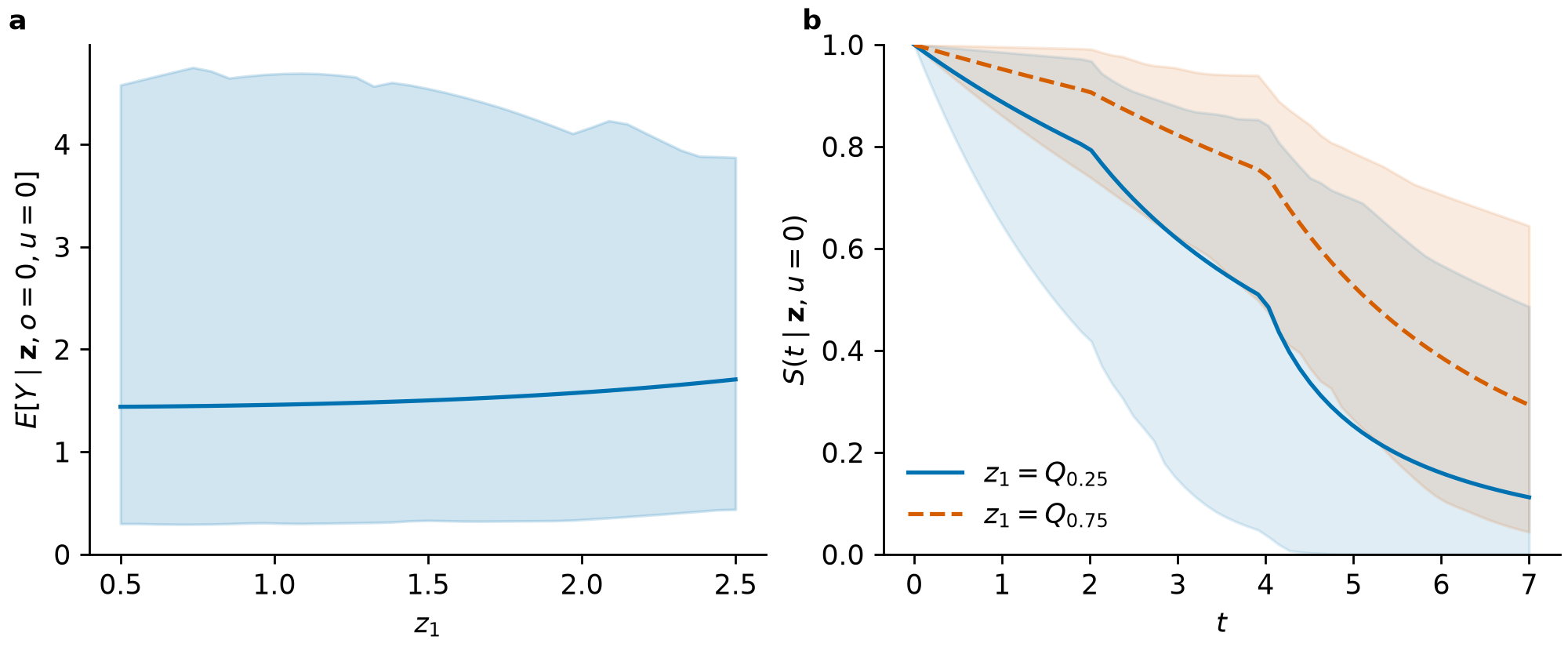
The figure uses the data above, 200 warmup and 200 saved draws per chain, two chains, and the same seeds. Predictions use 100 draws per chain. These short fits have mixing warnings and illustrate the outputs; they do not support inference or show whether the intervals achieve their stated coverage across repeated datasets. Figure values.

Account for clustered observations

Clustering can be modeled with any of the five outcome families. Supply cluster labels to identify observations that share a Gaussian random intercept. These labels group observations; exposure-selection groups instead groups exposure columns.

cluster = ["A"] * 3 + ["B"] * 3 + ["C"] * 3 + ["D"] * 3
clustered_fit = km.fit(
    counts, Z, family="poisson", cluster=cluster,
    draws=12, warmup=12, chains=2, seed=28,
)
intercepts = clustered_fit.random_intercepts(seed=29)
cluster_prediction = clustered_fit.predict(
    Z[:3], cluster_new=["A", "new", "new"], seed=29,
)

For a known cluster, prediction uses its fitted intercept. Rows with the same new label share one newly sampled intercept in each draw. Omitting cluster_new, or requesting exposure summaries, sets the intercept to zero; it does not average predictions over clusters. For slopes or Gaussian residual correlation, see structured models.

Plot the results

Plotting requires Matplotlib ([plots]). Each function returns an axes object; the caller controls display and export.

trace_ax = km.plot_trace(gaussian)
pip_ax = km.plot_pips(gaussian)
curve_ax = km.plot_response(curve)
overall_ax = km.plot_overall(overall)
surface_ax = km.plot_surface(surface)

# Optional: display the figures in an interactive session.
# import matplotlib.pyplot as plt
# plt.show()

Curve and overall plots show pointwise intervals. Surface plots show posterior means; result objects retain interval limits. Plot exposures separately when units differ. Traces exclude warmup.

Save and load a fit

A fit includes its retained training data as well as saved draws. Store and share it with the same care as the input data. The archive uses a non-pickle format.

from pathlib import Path
from tempfile import TemporaryDirectory

with TemporaryDirectory() as directory:
    path = Path(directory) / "mixture-fit.npz"
    gaussian.save(path)
    restored = km.BKMRFit.load(path)
    restored_prediction = restored.predict(Znew, Xnew, seed=20)

The API reference gives defaults, result fields and the definitions of pairwise interactions and median-reference centering. Method sources are Bobb et al. (2015) and the 2018 software and probit extension.