Ozone and weather in New York

We examine how daily ozone varies with solar radiation, wind and temperature, adjusting for month. This exploratory analysis uses the public New York air-quality data, separately from the applications in Bobb et al. (2015). Source data, saved results and sampling checks accompany the example.

Data and question

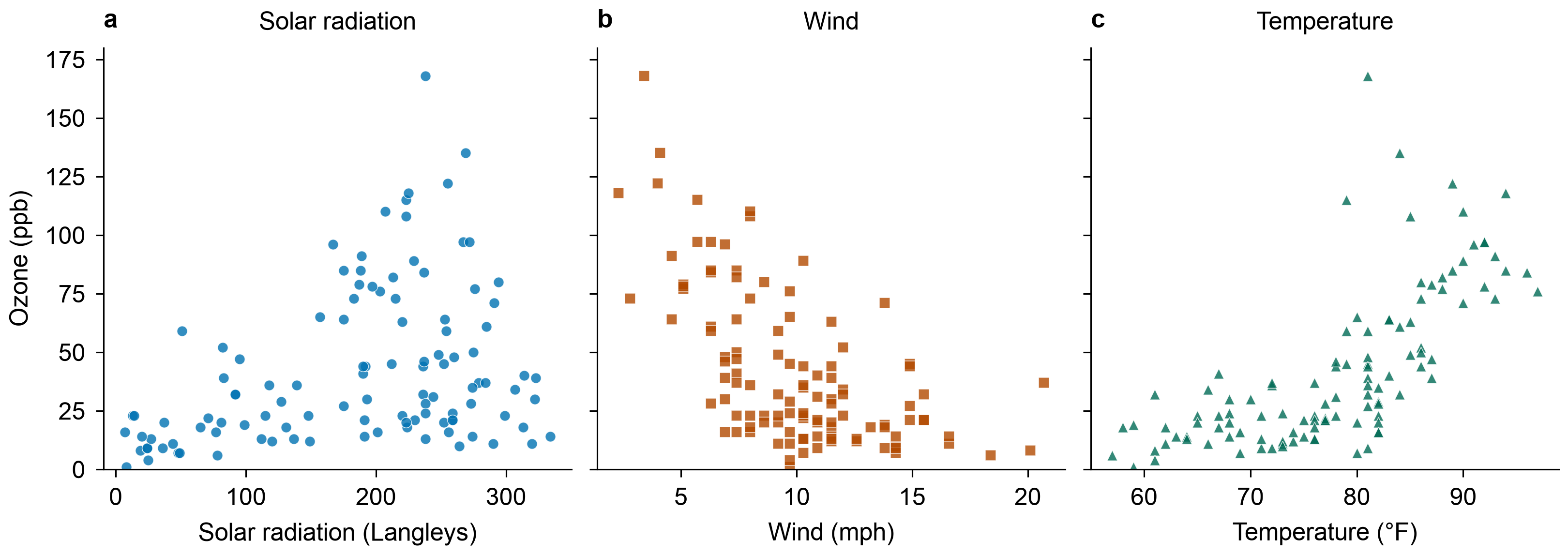
The R airquality data contain 153 daily records from New York, May–September 1973. Ozone was measured at Roosevelt Island, solar radiation at Central Park, and wind and temperature at LaGuardia Airport. Their measurement times also differ. These are daily environmental measurements, not personal exposures.

Variable	Role	Unit
`Ozone`	Outcome, transformed with the natural logarithm	Parts per billion
`Solar.R`	Exposure function	Langleys
`Wind`	Exposure function	Miles per hour
`Temp`	Exposure function	Degrees Fahrenheit
`Month`	Linear adjustment, May as reference	Four indicators

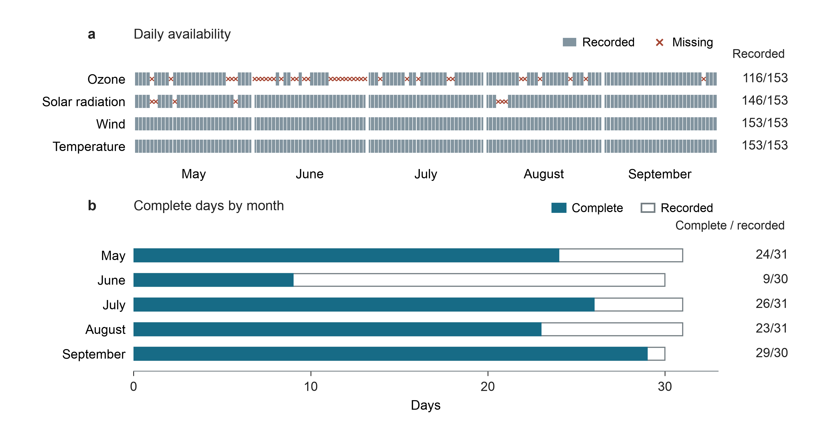
There are 37 missing ozone values and seven missing solar-radiation values. Keeping only rows with all required values retains 111 days and excludes 42. No missing values are filled in. The source CSV preserves all 153 records. Its provenance records the R version, hash, units and excluded row numbers.

Month	Recorded days	Complete days
May	31	24
June	30	9
July	31	26
August	31	23
September	30	29

Ozone medians are 31 ppb in complete rows and 35 ppb in the five rows missing solar radiation. Missingness is uneven across months, and ozone is unknown on 37 days. These observed ozone values do not show whether excluding incomplete days leaves the analysis unbiased.

Measurement availability among all 153 daily records. (a) Filled cells mark recorded measurements; crosses mark missing values. Fractions give recorded counts out of 153 days. (b) Filled bars show complete days within outlines for all recorded days, with complete/recorded counts. All four measurements are available on 111 days.

Observed ozone against solar radiation, wind and temperature for the 111 complete days. Each point is one day, without smoothing or adjustment for month.

Model and run

We use the Gaussian BKMR model with $Y_i=\log(\mathrm{Ozone}_i)$, $\mathbf z_i$ containing solar radiation, wind and temperature, and $\mathbf x_i$ containing an intercept and four month indicators:

\[Y_i=h(\mathbf z_i)+\mathbf x_i^\mathsf T\boldsymbol\beta+\epsilon_i,\qquad \epsilon_i\overset{\mathrm{iid}}{\sim}N(0,\sigma^2).\]

We standardize each exposure using the mean and sample standard deviation of the 111 retained days. Month indicators describe broad seasonality; independent errors remain a working assumption for this daily series.

For the Gaussian kernel, independent $r_m\sim\mathrm{Gamma}(1,1)$ priors use shape and rate one. Residual variance has an inverse-gamma(2,1) prior. We retain the default flat prior for adjustment coefficients and $\lambda=\tau/\sigma^2\sim\mathrm{Gamma}(1,0.1)$. Here $\tau$ is the GP covariance amplitude and $\sigma^2$ the residual variance. Exposure selection is disabled.

From the source folder, with KernelMix and its plotting extra installed:

python tools/analyze_airquality.py --draws 20000 --warmup 5000 --output ozone-results
python tools/plot_airquality.py --results ozone-results --output ozone-figure

Four chains run sequentially with seed 73. Each has 5,000 warmup iterations and 20,000 saved draws. An initial 4,000-draw run had maximum $\widehat R=1.0142$; one longer run was made to improve sampling, with the model, prior and data unchanged. This is an exploratory workflow, not a prospectively fixed study.

Results and checks

Check	Recorded result
Maximum rank/folded split $\widehat R$	1.0053
Minimum bulk effective sample size	885
Minimum tail effective sample size	1,193
Consecutive-day residual pairs	92
Correlation of consecutive-day fitted residuals	0.0136
Fitting time on the recorded local environment	72.6 seconds

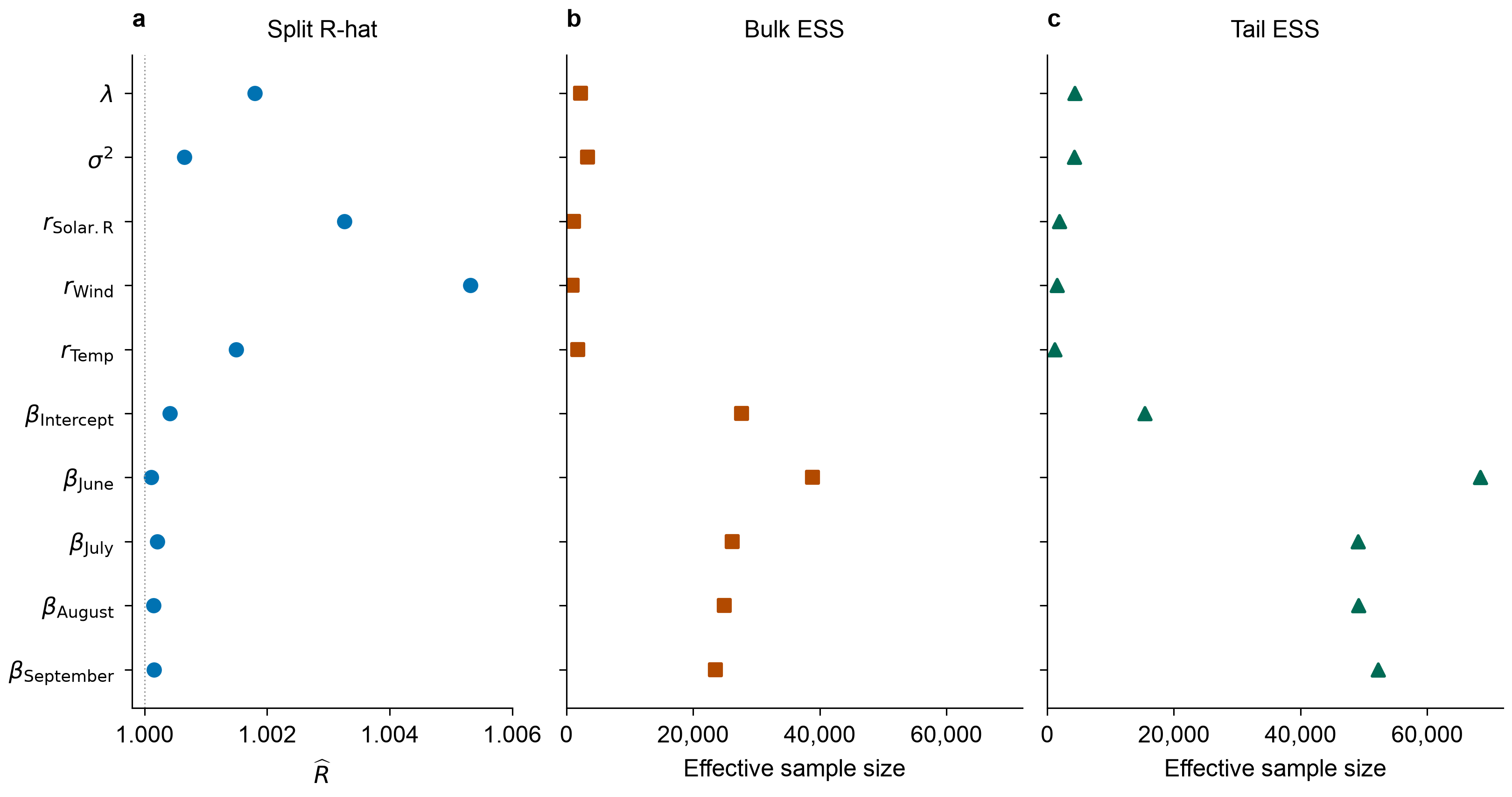
Sampling diagnostics use all saved draws for ten parameters. R-hat compares chains; effective sample size accounts for dependence between draws. These parameter diagnostics do not establish convergence of every estimated curve. Curve and fitted-residual summaries use 400 evenly spaced draws per chain.

Residual checks use training data, not held-out observations. The consecutive-day residual correlation cannot establish independent errors.

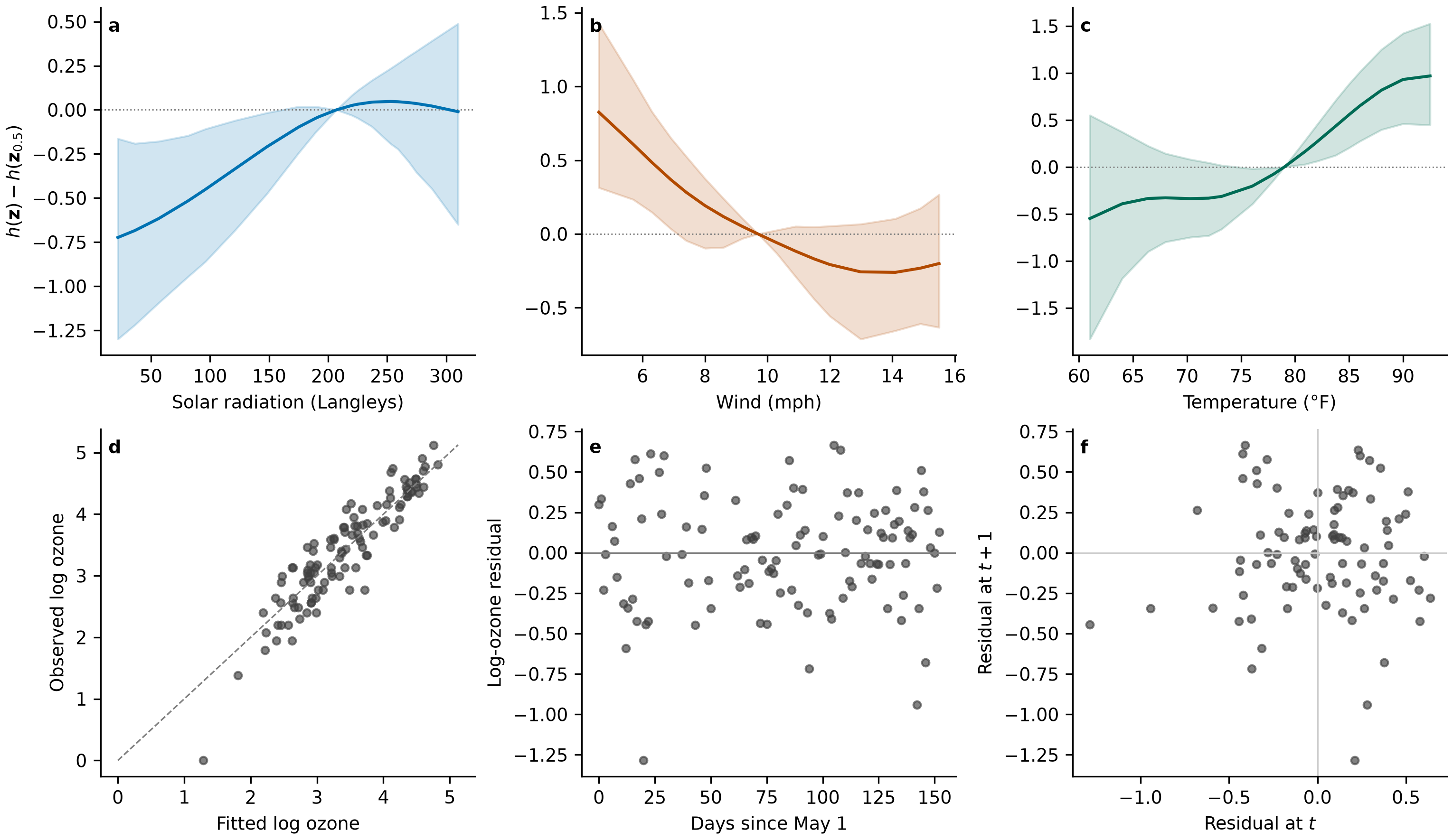
$Ozone example: (a–c) posterior means and 95% pointwise credible intervals for $h(\mathbf z)-h(\mathbf z_{0.5})$, with other exposures fixed at their sample medians and $\mathbf z_{0.5}$ the all-median profile; (d) fitted and observed log ozone; (e) residuals by date, with missing dates unconnected; (f) residual pairs one calendar day apart. Intervals assume independent Gaussian working errors.$

To isolate a conditional weather association, each curve varies one exposure with the others at their medians. The mean curve generally rises with temperature and falls with wind; the solar-radiation curve is nonlinear. On the log scale, exponentiating a difference gives a ratio of fitted ozone medians at fixed weather and month values, not an arithmetic mean difference.

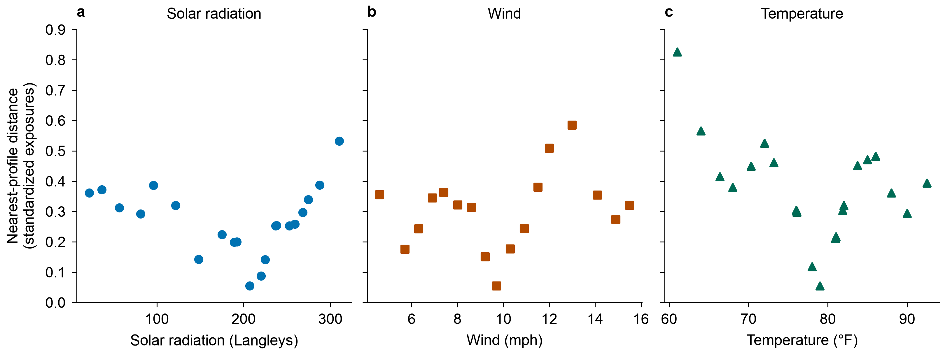
Each grid spans the 5th–95th percentiles, with duplicate values removed. Combining a grid value with the other exposures' medians may produce a profile uncommon in the observed data. The curve table records its distance to the nearest observed profile after standardization; the distance plot below shows how close these combinations are to the data.

Parameter estimates

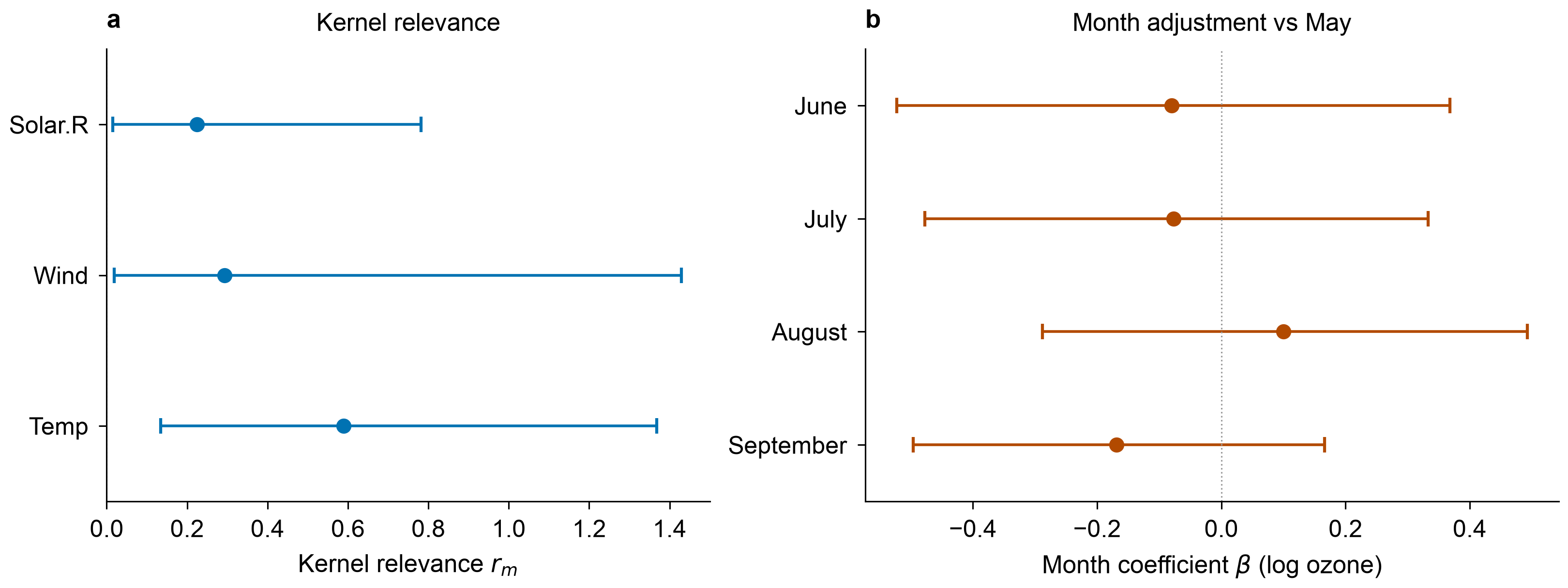
The kernel relevance parameters $r_m$ describe how exposure differences change the covariance of $h$. The month coefficients $\boldsymbol\beta$ instead describe differences from May on the log-ozone scale. Points show posterior means; bars show 95% equal-tailed credible intervals.

$Posterior means and 95% equal-tailed credible intervals. (a) Exposure relevance $r_m$. (b) Month coefficients in $\boldsymbol\beta$, relative to May, on the log-ozone scale. The intercept is omitted. Relevance does not measure causal importance.$

Sampling checks

To assess the sampling behind these intervals, we show diagnostics for all ten parameters. Bulk effective sample size concerns the center of the posterior; tail effective sample size concerns its tails.

$Sampling diagnostics from four chains, each with 20,000 saved draws. (a) Rank-normalized/folded split $\widehat R$. (b) Bulk effective sample size. (c) Tail effective sample size. These checks do not establish convergence or validate the model.$

Distance from observed exposure combinations

Sampling checks do not show whether a curve profile occurs in the data. We therefore measure its distance to the nearest observed profile, using training standard deviations to put exposures on a common scale. No distance cutoff establishes prediction reliability.

Nearest observed-combination distance along each saved curve grid, after standardizing exposures. Other exposures remain at their medians. There are 21 solar-radiation, 17 wind and 21 temperature locations; tied percentile values were removed. Distance describes data proximity, not model validity.

The plotting script regenerates these five additional figures from saved tables without refitting:

python tools/plot_airquality_details.py

Reuse and limits

The results record, parameter summaries, diagnostics, curve values and dated observations/residuals accompany the runnable scripts. R is not required to run the analysis. The source CSV was exported with R 4.5.0.

Missingness, measurement differences, priors and serial dependence limit interpretation. This example establishes neither causal effects nor time-series interval coverage. Original-study reproduction and external research use remain separate evidence gaps; see reference studies.