Overview

Author: Nilson Chapagain, Texas A&M University Email: nchapagain@tamu.edu

JointShrink estimates effects jointly across conditions using Gaussian mixture priors. The Gaussian summary-statistic method follows Urbut et al. (2019). Separate extensions support native multivariate Student-\(t\) summary likelihoods and direct regression from outcomes and predictors.

Input and model	Fitting method
Effect estimates and standard errors; Gaussian errors	Multivariate adaptive shrinkage (MASH), with empirical-Bayes mixture weights
Effect estimates and Student-\(t\) scale matrices	Native multivariate \(t\) likelihood, numerical quadrature and empirical-Bayes mixture weights
Outcomes and predictors	Gaussian-mixture coefficient prior with sampled coefficients and mixture weights; Gaussian, binomial, count, categorical and survival models

The direct-regression extensions use a different posterior model from Gaussian MASH. Their residual scales, dispersion, ordinal thresholds and Weibull shape are supplied and held fixed.

Installation

Python 3.10 or later is required.

pip install jointshrink

For Matplotlib plots and pandas tables:

pip install "jointshrink[plot,table]"

From GitHub

python -m pip install "git+https://github.com/nilson01/jointshrink.git@main"

From a local checkout

Run this command in the directory containing pyproject.toml:

python -m pip install .

NumPy and SciPy are required. Plots require Matplotlib; to_dataframe() requires pandas. Analysis does not require R.

Gaussian example

from jointshrink import set_data, fit

data = set_data([[1.2, 1.0], [-0.8, -1.0], [0.1, -0.2]], 0.5)
result = fit(data, scales=[0.25, 0.5, 1.0, 2.0])
print(result.format_summary())

Worked examples

Gaussian fitting with specified covariance patterns

Each row contains estimates of one effect across conditions; columns identify conditions. The following values are constructed examples.

import numpy as np
from jointshrink import set_data, fit, canonical_covariances

effects = np.array([
    [1.2, 1.0], [-1.1, -0.9], [0.1, -0.2],
    [1.5, 0.1], [-0.1, 1.4], [0.2, 0.1],
])
data = set_data(effects, 0.5, condition_names=["A", "B"])
patterns = canonical_covariances(data)
result = fit(data, patterns, scales=[0.25, 0.5, 1.0, 2.0])
print(result.format_summary())
print(result.posterior_mean)
print(result.interval(level=0.95))

posterior_mean estimates each effect after shrinkage. interval() returns equal-tailed marginal credible intervals. Both condition on the fitted covariance patterns and mixture weights. Check result.diagnostics["converged"] before interpreting a fit.

Covariance-pattern estimation

Strong rows help identify covariance patterns. Final mixture weights should instead use all rows or a representative training sample, because strong rows overrepresent large effects (Urbut et al., 2019).

from jointshrink import select_strong, cov_pca, cov_ed

strong = select_strong(data, z_threshold=2)
pca = cov_pca(data, n_components=2, subset=strong)
starts = {"PCA": pca["PCA_total"] + 0.1 * np.eye(data.n_conditions)}
learned = cov_ed(data, starts, subset=strong, maxiter=300)
patterns = {**canonical_covariances(data), **pca, **learned.covariances}
result = fit(data, patterns, scales=[0.25, 0.5, 1.0, 2.0])
print(learned.diagnostics["reason"])

Adding 0.1 makes this example's starting matrix positive definite; it is not a package default. Inspect the likelihood trace and stopping reason because covariance learning can reach a local optimum or its iteration limit.

Contrasts and effect sharing

contrast = result.contrast([[1, -1]], names=["A minus B"])
print(contrast.posterior_mean)
print(contrast.interval())
sharing = result.sharing(mode="magnitude", factor=0.5)
print(sharing["matrix"])
print(sharing["denominator"])

The contrast uses the joint posterior covariance. Magnitude sharing requires equal nonzero signs and posterior means within a factor of two. Each denominator counts rows with a selected error rate below the threshold in either condition. This proportion describes the fitted posterior means; it is not a posterior probability of sharing.

Posterior inference with a fitted prior

from jointshrink import fit_prior, save_prior, load_prior

prior = fit_prior(data, patterns, scales=[0.25, 0.5, 1.0, 2.0])
new_data = set_data([[0.8, np.nan], [-0.4, -0.6]], 0.5,
                    condition_names=["A", "B"])
new_result = prior.apply(new_data)
save_prior(prior, "prior.json")
restored = load_prior("prior.json")
for batch in restored.iter_apply(new_data, batch_size=128):
    print(batch.posterior_mean)

A missing effect estimate uses NaN; its standard error must still be finite and positive. The likelihood uses only the observed estimates and their sampling-covariance submatrix. The unobserved effect is inferred from the fitted prior and the observed effects. Retain the same condition order and EE/EZ scale; reuse holds patterns and weights fixed.

Student-t summary models

from jointshrink import set_data, fit_student_t

data_t = set_data([[1.2, 1.0], [-0.8, -1.0], [0.1, -0.2]], 0.5)
result_t = fit_student_t(data_t, df=4, scales=[0.25, 0.5, 1.0])
print(result_t.posterior_mean)
print(result_t.diagnostics["quadrature_converged"])

Here 0.5 is the square root of the Student-\(t\) scale diagonal, not the error SD. The native Student-t model explains the distinction.

Binomial regression

import numpy as np
from jointshrink import fit_logistic_regression

X = np.array([[-1.5], [-1.0], [-0.2], [0.3], [0.8], [1.4]])
y = np.array([0, 0, 1, 0, 1, 1])
regression = fit_logistic_regression(X, y, seed=4)
print(regression.format_summary())
print(regression.diagnostics["split_rhat"])
probability = regression.predict(X, scale="probability")

This constructed binary example has one predictor and an intercept. The result contains posterior draws; inspect the sampling diagnostics before interpretation. An estimated success probability differs from a sampled future binary outcome.

Plotting and result export

from jointshrink import plot_intervals, plot_sharing

ax = plot_intervals(result, condition="A")
ax.figure.savefig("intervals.png", dpi=300, bbox_inches="tight")
ax = plot_sharing(result)
records = result.to_records()
# With pandas installed:
table = result.to_dataframe()

Plot functions return Matplotlib axes and do not display or save figures automatically.

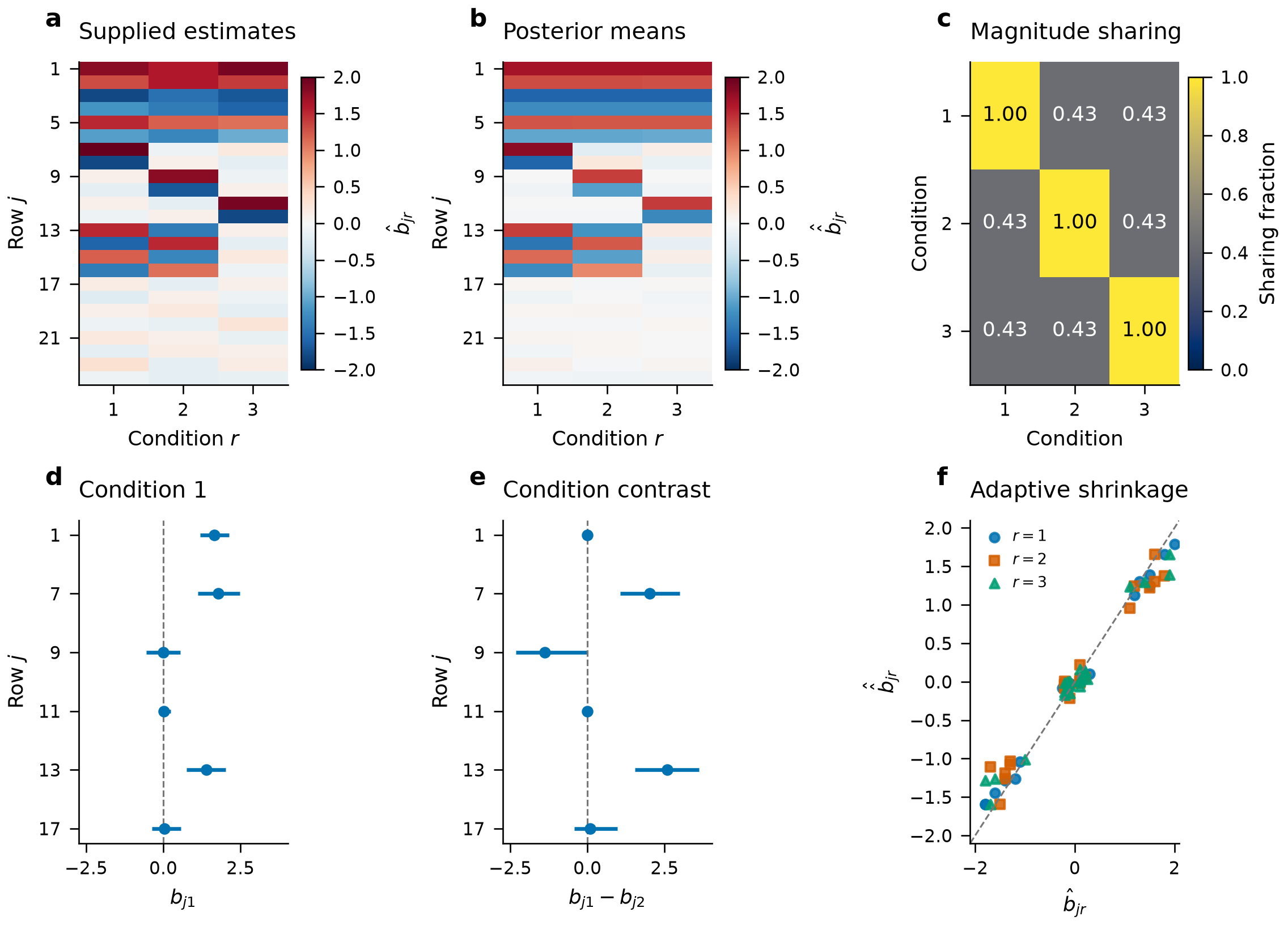
Model illustrations

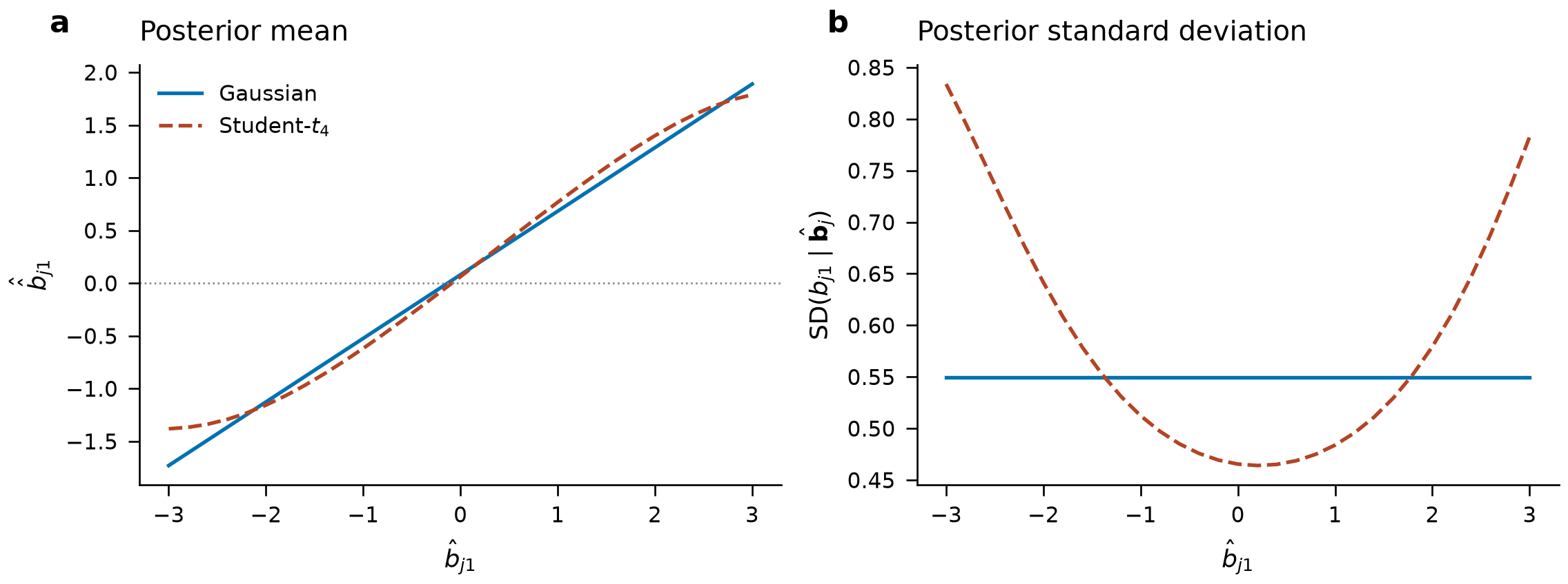
Both models use the same fixed prior and error covariance. For Student-\(t_4\) errors, the scale matrix is half that covariance. The second supplied estimate stays at \(0.5\) while the first varies. These are illustrations, not repeated-dataset comparisons. Input values and posterior summaries are available.

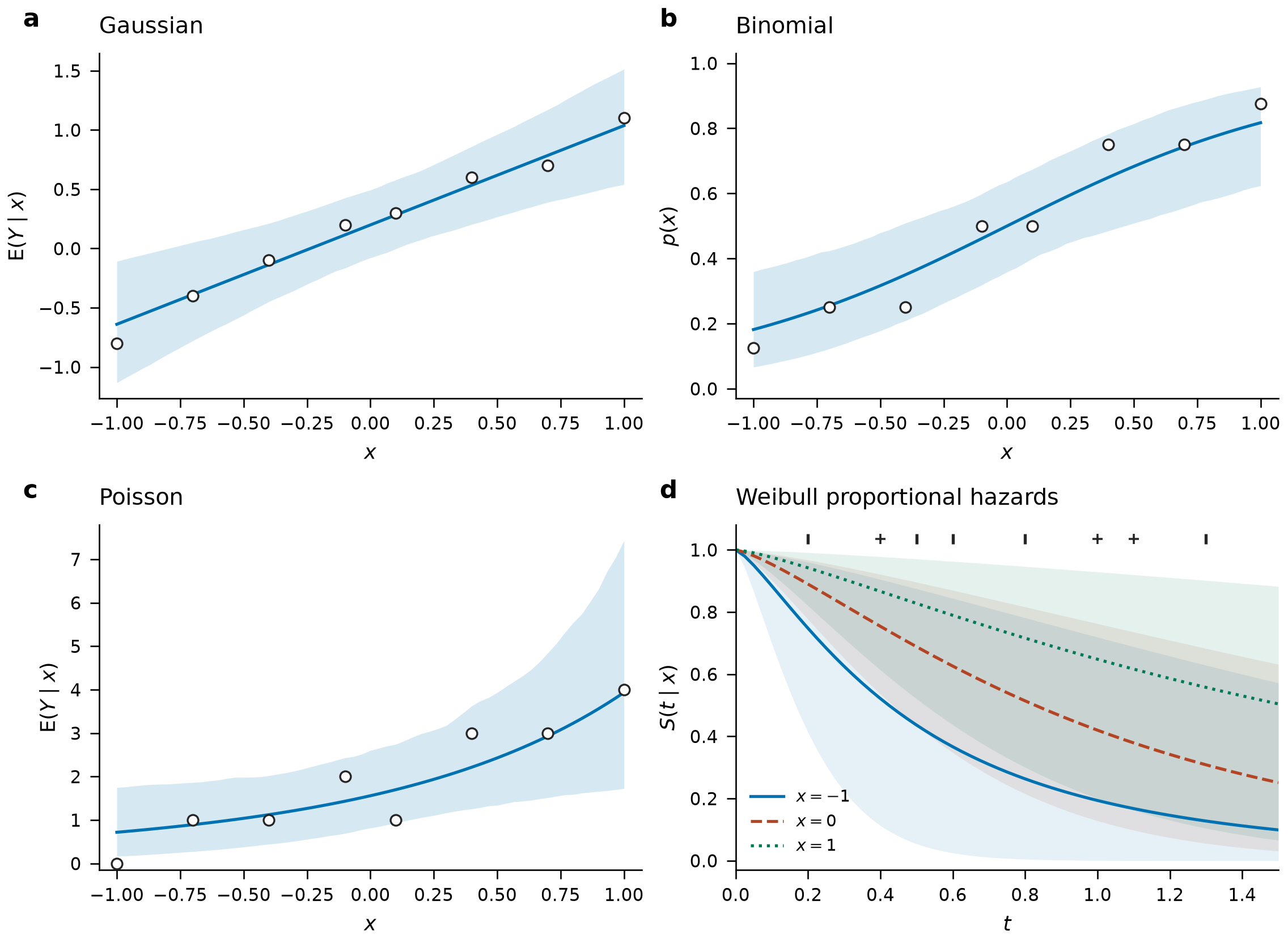
Each fit uses eight constructed observations, one predictor and two chains with 500 retained draws after 300 warmup iterations. Bands describe uncertainty in a conditional mean or survival probability, not future-outcome intervals. Gaussian residual SD is \(0.4\), binomial trials are 8, Poisson exposure is 2, and Weibull shape is 1.3. Inputs and predictions retain the plotted values.

Statistical models and inference

Gaussian summary model

Let \(b_{jr}\) be effect \(j\) in condition \(r\), and let \(\widehat b_{jr}\) and \(\widehat s_{jr}\) be its estimate and standard error. The vector \(b_j\) contains the true effects in \(R\) conditions. Following equations (2)–(4) of Urbut et al. (2019),

Here, \(N_R\) denotes an \(R\)-dimensional normal distribution (a density when its covariance is positive definite), \(V_j\) is the observation-error covariance, \(U_k\) describes an effect-sharing pattern, \(\omega_l\) multiplies its covariance, and \(\pi_{k,l}\) is a mixture proportion. The proportions are nonnegative and sum to one. The covariance patterns are positive semidefinite (PSD). Consequently,

Observation-error matrices must be positive definite. Prior patterns may be singular, including a point mass at zero. Rows are treated as independent when fitting the mixture likelihood.

Effect scales and observation errors

alpha=0 fits exchangeable effects (EE): the common prior describes effects in their original units, independently of the supplied standard errors. alpha=1 fits exchangeable Z scores (EZ): the common prior instead describes effects divided by their standard errors. EZ fitting divides both the estimates and their sampling errors by those standard errors. Posterior summaries are returned in the original effect units. Original-scale log densities include the transformation Jacobian for observed coordinates.

With supplied standard errors and error correlation \(C\), the model uses \(V_j=S_j C S_j\), where \(S_j\) has diagonal entries \(\widehat s_{jr}\). error_covariance supplies \(V_j\) directly and replaces both standard errors and correlation inputs. estimate_null_correlation estimates correlation from complete rows with all absolute Z scores below a threshold; selection can bias this estimate.

Missing effect estimates use NaN. Their standard errors remain required, including under EZ, to define the output scale. Likelihoods use observed-condition blocks of \(V_j\); posterior inference can include unobserved conditions. This does not correct informative missingness. PCA and extreme-deconvolution learning require complete selected rows.

Covariance patterns and scale grids

Canonical patterns describe effects that, within a Gaussian component, are uncorrelated, nonzero in one condition, equal across conditions, or positively correlated. A mixture of diagonal-covariance components need not make the effects marginally independent. Principal component analysis (PCA) supplies candidate directions from strong rows. Its default uses an uncentered singular value decomposition (SVD) of working effect estimates, following the R helper. Centered Z-score PCA requires alpha=1 and center=True.

Extreme deconvolution fits a zero-mean Gaussian mixture while accounting for observation error, following the noisy-mixture approach used by Urbut et al. (2019). The algorithm can have local optima. An exactly singular start cannot expand its support under unconstrained expectation–maximization (EM) updates. ridge sets an explicit eigenvalue floor; rank limits component rank. Projected proposals are accepted only when the observed likelihood does not decrease. A rejected proposal and an iteration limit are reported separately from convergence.

Patterns are normalized by their largest diagonal entry unless normalize=False. Python scales contains standard-deviation multipliers: their squares are the paper's covariance multipliers \(\omega_l\). The automatic grid spans small working standard errors through the largest observed working effect. Use an explicit grid when matching another implementation.

Mixture-weight estimation and posterior uncertainty

fit_prior estimates mixture weights using the supplied rows. null_weight=1 uses maximum likelihood; larger values add a log-weight penalty favoring the global-null component. A penalized fit requires that component. Inspect the convergence flag, objective trace and Karush–Kuhn–Tucker (KKT) residual in the fitted diagnostics. A small KKT residual checks the weight-optimization conditions, not the observation model.

Posterior means, credible intervals and sign probabilities condition on the selected patterns and fitted weights. They do not include all uncertainty from learning those quantities. For each effect and condition,

The local false sign rate includes zero mass in either possible sign error. lfdr is the marginal posterior probability of an exact zero. joint_null_probability concerns the entire row being zero. The displayed probabilities hold fitted prior parameters fixed. These probabilities depend on the observation model and fitted prior.

Memory management

A full result stores component-specific posterior covariance matrices. Storage therefore grows with rows × components × conditions squared. The kernel rejects a posterior-component allocation above 256 MiB; total process memory can be higher. Use fit_prior for weight fitting and prior.iter_apply(data, batch_size=...) for ordered posterior batches. Scoring and prior fitting use likelihood-only calculations. Reduce the batch size when the number of conditions or components is large.

Retain the original condition order when reusing a prior: columns are matched positionally. prior.apply is the Gaussian summary interface; native \(t\) reuse requires apply_student_prior or StudentTResult.shrink. FLASH/UDR covariance learning and GPU fitting are not provided.

Native Student-t summary model

For estimates with heavier-tailed errors, the native \(t\) route retains the Gaussian mixture prior but changes the observation model. Here \(V_j\) denotes a positive-definite error scale matrix, rather than the Gaussian sampling covariance. Let \(\nu_j>0\) be the supplied degrees of freedom. The implementation uses

One precision \(\lambda_j\) is shared across a row's observed conditions. This gives elliptical multivariate \(t\) errors, rather than independent univariate \(t\) errors. The scale convention follows SciPy's multivariate \(t\) definition. The error covariance is \(\nu_j V_j/(\nu_j-2)\) only for \(\nu_j>2\); it does not exist for \(\nu_j\leq2\).

For this route, error_covariance supplies \(V_j\), and standard_errors supplies its diagonal square roots when an explicit scale matrix is not supplied. These inputs are not error standard deviations under a finite-degree-of-freedom \(t\) likelihood. EE/EZ transformations retain the same original-scale Jacobian as Gaussian MASH. Missing conditions use the observed block of \(V_j\).

Integration over log precision produces a finite Gaussian-mixture approximation to the posterior. Increasing quadrature orders checks marginal log densities, first and second posterior moments, and CDFs at zero. Inspect quadrature_converged and quadrature_relative_change; an unmet tolerance produces a warning. These checks are not rigorous error bounds for every posterior quantile. Uncertainty remains conditional on supplied \(V_j,\nu_j\) and fitted prior parameters.

Regression models

Direct regression starts from outcomes, rather than estimates from an earlier analysis. Let \(X\) contain \(n\) observations and \(p\) predictors, and let \(D\) be the number of linear predictors needed by the likelihood. Each coefficient row \(B_j\in\mathbb R^D\) has the same mixture prior. The covariance components describe relationships among its \(D\) linear-predictor coefficients; mixture weights are shared across the \(p\) predictor rows:

The fixed matrices \(\Sigma_k\) include supplied covariance patterns and squared SD multipliers; a zero component is included when point_mass=True. dirichlet supplies positive concentrations \(a_k\). Unlike fit_prior, this model samples \(\pi\) rather than maximizing a marginal likelihood.

With intercept \(\beta_{0r}\), supplied offset \(o_{ir}\) and group effects \(u_{g(i),qr}\), its linear predictor is

Group terms are absent when groups=None. Intercepts have independent \(N(0,5^2)\) priors; Cox models omit them. Inputs are not standardized automatically, so predictor and response units affect these priors. Use the same predictor order and preprocessing for fitting and prediction. Constant or aliased predictors can prevent separate coefficients from being identified by the likelihood, even with proper priors.

Outcome distributions and link functions

Except for the single categorical or survival outcome, y can have shape (n,R). Its columns are conditionally independent given their predictors and group effects. Shared coefficient or group priors do not provide a general residual covariance model. Missing raw outcomes and predictors are rejected.

Let \(\mathrm{logit}^{-1}(x)=1/(1+e^{-x})\). For the negative binomial, NB2 denotes the variance convention given below. In count models, \(e_{ir}>0\) is supplied exposure and \(\mu_{ir}=e_{ir}\exp(\eta_{ir})\) is the mean of the underlying Poisson or NB2 count component. In zero-inflated and hurdle models, the overall response mean differs from \(\mu_{ir}\).

family	Likelihood and supplied quantities
gaussian	\(y_{ir}\sim N(\eta_{ir},\sigma_{ir}^2)\); positive sigma fixed
binomial	\(y_{ir}\sim\mathrm{Binomial}(m_{ir},\mathrm{logit}^{-1}(\eta_{ir}))\); integer trials supplies \(m_{ir}\); binary outcomes use one trial
poisson	\(y_{ir}\sim\mathrm{Poisson}(\mu_{ir})\)
negative_binomial	NB2 with mean \(\mu_{ir}\) and variance \(\mu_{ir}+\phi_{ir}\mu_{ir}^2\); positive dispersion supplies fixed \(\phi_{ir}\)
multinomial	One category vector coded \(0,\ldots,K-1\); \(K-1\) logits with category \(K-1\) as reference
ordinal	\(\Pr(y_i\leq k\mid\eta_i)=\mathrm{logit}^{-1}(c_k-\eta_i)\) for \(k=0,\ldots,K-2\); strictly ordered thresholds \(c_k\) fixed
cox	Proportional hazards with Breslow tied-event partial likelihood; event and positive observed times required
weibull	Proportional hazards with baseline cumulative hazard \(H_0(t)=t^a\); positive shape \(a\) fixed

Categorical models infer the category count from observed codes unless n_categories is supplied. Supply it when unobserved categories must be retained. Ordinal default thresholds are the logits of \(1/K,\ldots,(K-1)/K\); they are not estimated. Increasing the ordinal predictor shifts mass toward larger category codes. This cumulative-link convention is described in the statsmodels ordered-model reference.

Zero-inflated and hurdle models

zero_inflated_poisson, zero_inflated_negative_binomial, hurdle_poisson and hurdle_negative_binomial use \(2R\) linear predictors: count predictors first, then zero-probability logits. Write \(\rho_{ir}\) for the inverse-logit of the second predictor and \(f(y;\mu,\phi)\) for the Poisson or NB2 mass.

Thus the zero-inflated mean is \((1-\rho)\mu\), while the hurdle mean is \((1-\rho)\mu/[1-f(0)]\). The zero logit has the same direction in both models: larger values increase zero probability. By default these fits use an identity covariance pattern for coefficients across the count and zero predictors; supplied patterns may express a chosen relationship.

Survival models

Both survival families support right censoring and delayed entry with 0 <= entry < time. The Cox risk set at event time \(t\) uses \(\mathrm{entry}_i<t\leq\mathrm{time}_i\), with Breslow handling of tied events. The coefficient posterior is proportional to the Cox partial likelihood times the specified priors; it does not come from a full event-time likelihood. Survival inference requires non-informative censoring conditional on the modeled predictors and group effects, and appropriate adjustment for delayed entry. Absolute survival uses a draw-specific Breslow baseline estimated from the training data; it propagates coefficient uncertainty but does not integrate separate baseline uncertainty. No-event data cannot supply an absolute baseline. The statsmodels PHReg reference describes the corresponding right-censoring, entry and ties conventions. Weibull absolute survival instead depends on the supplied shape and parametric baseline. Competing risks, interval censoring and time-varying covariates are not included.

Gaussian random effects

groups supplies one nonempty string label per observation. Without random_design, each group has a random intercept. A supplied (n,Q) design allows random slopes. Flattening each group's (Q,D) effects in row order gives

random_covariance supplies the fixed positive-definite shape matrix \(A\) of dimension (Q*D,Q*D). The default is identity. random_scale supplies the common multiplier \(\tau\); marginal group-effect SDs also depend on the diagonal of \(A\). With estimate_random_scale=True, it sets the initial value and \(\tau^2\) has an inverse-gamma prior with shape 2 and scale 1. Otherwise it stays fixed. This estimates one common scale, not an unrestricted random-effect covariance or general within-group residual correlation.

Posterior sampling and convergence diagnostics

Regression uses Markov chain Monte Carlo (MCMC). It combines joint component/coefficient proposals from the current prior, elliptical slice updates within Gaussian components, and Dirichlet updates for mixture weights. Elliptical slice sampling follows Murray, Adams and MacKay (2010). Component-changing proposals allow transitions between zero, singular and full-rank prior components. A failed slice-bracket search raises an error rather than accepting an approximate update.

Inspect coefficient traces, split_rhat, effective_sample_size, constant_coordinates, prior_proposal_acceptance and component_switches. The effective sample size is an autocorrelation estimate, not a rank-normalized bulk effective sample size. Constant coordinates have undefined diagnostics; a chain stuck at zero is not evidence of convergence. The coefficient diagnostics do not certify mixing for every group effect or mixture weight. Successful execution and multiple chains do not establish convergence or calibration.

API reference

All functions below are imported from jointshrink. Summary arrays use effects × conditions, with (n,d) denoting rows × conditions in API shapes. Regression uses observations × predictors; \(D\) denotes its number of linear predictors.

Summary-statistic inputs

set_data(effects, standard_errors=1, *, correlation=None,
         error_covariance=None, alpha=0, row_names=None, condition_names=None)

Returns MashData. effects has shape (rows, conditions) with at least two conditions; NaN marks a missing estimate. Standard errors broadcast to that shape and must be finite and positive. Correlation or explicit sampling covariance can be shared (d,d) or row-specific (n,d,d). Explicit covariance cannot be combined with correlation or nondefault standard errors. alpha is 0 (EE) or 1 (EZ).

MashData.subset(indices) selects rows and preserves covariance and scale information. Input arrays are copied and exposed read-only. Row and condition names must be unique.

Covariance patterns

Function	Purpose and main controls
canonical_covariances(data_or_dimension, *, methods=...)	Identity, singletons, equal effects and simple heterogeneous patterns; null is also available
validate_covariances(patterns, *, normalize=False)	Named PSD matrices; maximum-diagonal normalization when requested
select_strong(data, *, z_threshold=3)	Row indices with an observed absolute Z score above the threshold
cov_pca(data, n_components=2, *, subset=None, center=False)	Rank-one PCs and their aggregate; complete selected rows required
cov_ed(data, initial, *, subset=None, maxiter=200, tol=1e-6, ridge=0, rank=None)	Error-aware covariance refinement; returns CovarianceFit
make_scale_grid(data, *, factor=sqrt(2))	Positive standard-deviation grid
expand_covariances(patterns, scales, *, point_mass=True, normalize=True)	Pattern × squared-scale combinations, deduplicated
estimate_null_correlation(data, *, z_threshold=2, minimum_rows=None, regularization=0.05)	Correlation of centered Z scores in rows below the absolute-Z threshold, shrunk toward identity

CovarianceFit exposes covariances, weights and diagnostics. Its likelihood history and stopping reason distinguish convergence from an iteration limit or rejected proposal. CorrelationEstimate exposes correlation, selected row_indices and diagnostics.

Gaussian fitting and prior reuse

fit_prior(data, covariances=None, *, scales=None, normalize=True,
          point_mass=True, null_weight=1, initial_weights=None,
          maxiter=10000, tol=1e-8)
fit(data, covariances=None, **options)

Both functions fit mixture weights on all supplied rows. Omitted patterns use canonical covariances; omitted scales use the automatic grid. scales are SD multipliers. fit_prior returns MashPrior without allocating posterior moments. fit accepts the same options and returns MashResult. Mash(covariances=None, **options).fit(data) provides the configured-fit interface.

Prior interface	Behavior
MashPrior(covariances, names, weights, *, alpha=0, metadata=None)	Construct a validated prior from already expanded covariance matrices and weights summing to one
prior.apply(data) or apply_prior(data, prior)	Condition on new rows without refitting
prior.iter_apply(data, *, batch_size=128)	Yield posterior batches in row order
prior.score_samples(data) or score_samples(data, prior)	Per-row log density in observed original units

A reused prior requires the same condition order, number of conditions and EE/EZ scale. Stored prior covariances are already expanded; reuse does not apply a second scale grid.

Posterior summaries

MashResult extends PosteriorResult with prior, data, diagnostics, per-row log_likelihood, and log_bayes_factor. The Bayes factor compares the fitted nonnull mixture, renormalized to nonnull weight one, against the global null. A result with no nonnull prior weight has log Bayes factor -inf.

Property	Shape or meaning
posterior_mean, posterior_sd	(n,d)
posterior_covariance	(n,d,d)
lfdr, lfsr	(n,d); marginal posterior null probabilities and local false sign rates
probability_negative, probability_positive	Strictly negative/positive posterior probability
joint_null_probability	(n,); all conditions exactly zero
row_names, condition_names, observed	Labels and observed-coordinate mask

Method	Result
cdf(value)	Marginal probability of effect \(\leq\) value
quantile(probability)	(n,d) for scalar probability; (p,n,d) for a vector
interval(level=0.95)	Equal-tailed intervals, (n,d,2)
sample(size=1, seed=None)	Conditional posterior draws, (size,n,d)
contrast(coefficients, *, names=None)	Joint posterior for linear contrasts; coefficients have shape (contrasts,d)
significant(threshold=0.05, *, by="lfsr", any_condition=True)	Row indices selected in any condition, or all when False
sharing(*, factor=0.5, threshold=0.05, by="lfsr", mode="magnitude")	Posterior-mean sharing matrix plus numerator, denominator and definition
to_records(*, level=0.95)	Long-form Python records
to_dataframe(*, level=0.95)	pandas table; requires pandas
summary(*, threshold=0.05, by="lfsr")	Compact dictionary
format_summary(*, threshold=0.05, by="lfsr")	Readable summary text

MashResult.shrink(data) reuses its prior. score_samples(data) evaluates new rows. Uncertainty conditions on the fitted patterns and weights.

Student-t fitting

fit_student_t(data, df, covariances=None, *, scales=None, normalize=True,
              point_mass=True, null_weight=1, initial_weights=None,
              quadrature_order=64, max_quadrature_order=256,
              quadrature_tol=1e-5, maxiter=10000, tol=1e-8)
apply_student_prior(data, prior, df, *, quadrature_order=64,
                    max_quadrature_order=256, quadrature_tol=1e-5)

df is required: finite positive scalar or one value per effect row. Infinite df is not accepted; use Gaussian fit for Gaussian errors. Quadrature orders are integers of at least four, with maximum no smaller than the starting order. A single unrefined order reports convergence as unverified.

StudentTResult inherits the posterior methods above and adds data, prior, df, log_likelihood and diagnostics. Its Gaussian-mixture effect prior can be saved independently. Use result.shrink(new_data, df=...) for native \(t\) reuse; prior.apply would use a Gaussian likelihood. Quadrature nodes increase the number of stored posterior components, so fewer rows or patterns may be needed within the 256 MiB component guard.

Regression fitting

fit_regression(X, y, *, family="gaussian", covariances=None,
               scales=(0.1, 0.5, 1, 2), point_mass=True,
               draws=1000, warmup=500, chains=4, seed=0,
               fit_intercept=True, offset=0, groups=None,
               random_design=None, random_covariance=None,
               random_scale=1, estimate_random_scale=True, dirichlet=1,
               coefficient_names=None, outcome_names=None, **likelihood_options)

X is a finite numeric (n,p) matrix. Gaussian, binomial and count y accepts (n,) or (n,R); categorical and survival models take a single outcome vector. There is no formula parser or automatic encoding of predictor categories. Encode them before fitting and preserve that encoding for prediction. offset broadcasts to observations by linear predictors. chains >= 2, draws >= 4 and warmup >= 0 are required.

Unlike summary-pattern fitting, regression does not normalize supplied covariance patterns. scales multiplies their SDs in the supplied predictor units. Omitted patterns use canonical patterns when the latent dimension exceeds one, except excess-zero models default to identity. The retained-draw allocation guard is 512 MiB, not a total process-memory limit.

Family-specific wrapper	Required or useful likelihood inputs
fit_gaussian_regression(X, y, **options)	sigma=1, scalar or broadcastable residual SDs, held fixed
fit_logistic_regression(X, y, **options)	trials=1; successes cannot exceed integer trials
fit_poisson_regression(X, y, **options)	Positive exposure=1
fit_negative_binomial_regression(X, y, **options)	Positive exposure=1, fixed dispersion=1
fit_multinomial(X, y, **options)	Integer codes; n_categories retains absent categories
fit_ordinal(X, y, **options)	Category codes and fixed ordered thresholds
fit_zero_inflated_poisson, fit_hurdle_poisson	(X,y,**options); positive exposure
fit_zero_inflated_negative_binomial, fit_hurdle_negative_binomial	(X,y,**options); positive exposure and fixed dispersion
fit_survival(X, time, event, *, family="cox", **options)	event required; entry=0; Cox ties="breslow"; Weibull fixed shape=1

make_likelihood(y, family=..., **likelihood_options) constructs a fixed-parameter Likelihood without regression fitting. loglike(eta) accepts (n,D) linear predictors. predict, sample and to_dict provide conditional prediction, outcome generation and reconstruction inputs. Unsupported family controls raise errors.

Regression results and prediction

RegressionResult extends DrawResult. Its main arrays are draws with shape (chains,draws,p,D), intercept_draws (chains,draws,D), weight_draws (chains,draws,K) and random_draws (chains,draws,groups,Q,D). random_scale_draws stores the retained common multiplier \(\tau\); the supplied covariance shape determines individual group-effect SDs. posterior_mean and coefficients contain the coefficient means; intercept gives intercept means.

DrawResult supplies posterior_sd, posterior_covariance, lfdr, lfsr, joint_null_probability, cdf, quantile, interval, sample, contrast, summary, format_summary, to_records and to_dataframe. These summaries are Monte Carlo estimates from retained posterior draws. sample resamples retained draws; it does not run more MCMC. Contrasts combine the last, latent-predictor dimension, rather than predictor rows. random_effect_summary(level=0.95) returns records for group intercepts/slopes.

result.predict(X, *, scale="response", groups=None, random_design=None,
               offset=0, allow_new_groups=False, seed=0, **options)
result.predict_interval(X, *, level=0.95, scale="response", **options)
result.posterior_predictive(X, *, seed=0, **options)

Predictions transform each retained linear predictor before averaging. predict_interval describes posterior uncertainty in the conditional mean or probability; posterior_predictive adds future-outcome variation.

scale	Prediction
"link"	Linear predictors, before adding count exposure; includes zero-probability logits where applicable
"response"	Expected response; categorical probability vector; survival relative hazard
"probability"	Binomial success probability or categorical probabilities
"relative_hazard"	Cox or Weibull relative hazard
"survival"	Cox or Weibull survival, with time required
"cumulative_hazard"	Weibull cumulative hazard, with time required

Supply new trials, exposure and offset explicitly when they differ from their defaults of one, one and zero. Training-row offsets are not reused. Row-specific fixed sigma or dispersion cannot be transferred to a different prediction row count; use a common supplied value for such prediction workflows.

Known groups use their retained group effects. With groups=None, the group effect is zero; under nonlinear links this is not the population-marginal response mean. Unknown labels require allow_new_groups=True, which draws Gaussian effects using each retained common scale. Repeated new labels share the same group draw; supply the matching new random-slope design.

Cox survival accepts a scalar or vector of times, returning (new_rows,times), and estimates the Breslow baseline separately for each retained coefficient draw. Its intervals still omit separate baseline uncertainty. Cox future event-time draws are unavailable. Weibull survival instead accepts scalar or per-row times. Weibull future-time draws are uncensored event times; a censoring process is not generated.

Plotting functions

Function	Display
plot_covariances(prior_or_mapping, *, axes=None, ncols=3, condition_names=None)	Covariance patterns
plot_weights(prior_or_result, *, ax=None)	Fitted mixture weights
plot_sharing(result, *, factor=0.5, threshold=0.05, by="lfsr", mode="magnitude", ax=None)	Descriptive sharing matrix
plot_intervals(result, *, condition=0, indices=None, level=0.95, ax=None)	Marginal posterior means and intervals
plot_diagnostics(result_or_covfit, *, ax=None)	Fitting objective or covariance-learning likelihood
plot_effects(result, condition=0, *, ax=None)	Supplied estimates and posterior means

For direct regression, plot_coefficients(result, *, condition=0, level=0.95, ax=None) shows coefficient intervals; plot_chains(result, *, term=0, condition=0, ax=None) shows retained traces. plot_regression_weights(result, *, level=0.95, ax=None) displays sampled mixture proportions, and plot_random_effects(result, *, condition=0, level=0.95, ax=None) displays group effects. Use the trace plot to inspect sampling behavior.

Plots require Matplotlib and return axes. They do not change global style or save files automatically.

Data and result persistence

save_data(data, path, *, overwrite=False)
load_data(path)
save_prior(prior, path, *, overwrite=False)
load_prior(path)
save_result(result, path, *, overwrite=False)
load_result(path)

These functions use schema-checked JSON rather than pickle. Existing files require overwrite=True. Gaussian loading reapplies the saved prior; native \(t\) loading repeats quadrature with the saved df and settings. Neither refits mixture weights. load_student_result(path) loads a native \(t\) result explicitly; generic save_result and load_result also retain that likelihood.

For regression, use save_regression_result(result, path, *, overwrite=False) and load_regression_result(path), or result.save(path). Loading restores retained draws without sampling. These files include training predictors, outcomes, group labels and offsets as well as posterior draws; treat them as analysis data.

Numerical reference checks

The reference checker compares the Gaussian workflow with installed R mashr 0.2.79. Fixed cases cover EE and EZ, supplied and estimated mixture weights, null-biased fitting, and explicit scale expansion. Compared outputs include posterior means, standard deviations, covariances, local false sign rates and local false discovery rates. An uncentered PCA comparison checks the matched helper convention.

The reference export records package versions and library origin. The checker uses absolute and relative tolerances of 2e-10 for fixed-prior cases and 2e-5 for fitted-weight cases. PCA matrices use 1e-12. See tools/export_mashr_reference.R and tools/check_mashr_reference.py in the repository.

Reference conventions and comparison limits

Area	Interpretation
Missing conditions	Python uses exact observed-block Gaussian likelihoods; R's large-SE substitution is an approximation
PCA	Match EE/EZ preprocessing, centering and selected rows before comparing matrices
Scales	Python inputs are SD multipliers; covariance multipliers are their squares
Covariance learning	Independent analytic checks cover noisy-mixture updates; an installed-R extreme-deconvolution comparison is not claimed
Uncertainty	Numerical agreement does not establish repeated-dataset coverage or include all hyperparameter uncertainty

R mashr finite-degrees-of-freedom inputs use normal-score conversion. JointShrink's native \(t\) likelihood and direct-regression extensions are separate methods; the Gaussian R comparisons do not validate them. Independent finite-case checks cover \(t\) convolution, outcome densities and masses, Cox partial likelihood, analytic regression posteriors and prediction behavior. Repeated-dataset coverage, general sampler mixing and full paper reproduction are not established by those checks.

Frequently asked questions

Does analysis require R?

No. NumPy and SciPy perform analysis. R is used only for Gaussian reference checks.

Does the package fit outcomes and predictors directly?

Yes. fit_regression(X, y, family=...) uses raw outcomes and a shared Gaussian-mixture coefficient prior. This sampling model differs from empirical-Bayes summary fitting. Supply and justify its fixed residual scales, dispersion, thresholds or Weibull shape where required.

Are credible intervals frequentist confidence intervals?

They are marginal posterior credible intervals. Summary fits condition on fitted prior parameters; direct regression samples coefficients and mixture weights but holds specified likelihood parameters fixed. Regression intervals also have Monte Carlo error. Repeated-dataset coverage requires a separate statistical evaluation.

Can estimates be missing?

Summary fitting allows NaN effects with positive finite standard errors for every coordinate. Each row needs an observed condition, and pattern learning requires complete selected rows. Direct regression requires complete predictors and outcomes.

Why did a fit stop without convergence?

Gaussian weight fitting reports an objective and KKT residual. Covariance learning reports its stopping reason. Native \(t\) fitting adds quadrature diagnostics, while regression reports chain and proposal diagnostics. A result object alone does not establish convergence.

Why is a sharing entry NaN?

No rows met the selection threshold in either condition, so the denominator is zero. Sharing summarizes posterior means; it is not a posterior probability that two effects are equal.

How can memory use be reduced?

Use fit_prior and iterate over prior.iter_apply(data, batch_size=...). Reduce the batch size when there are many conditions or components. The posterior tensor guard is not a total process-memory limit.

License and attribution

JointShrink is distributed under GPL-3.0-or-later. See LICENSE for the license terms. The statistical method and the R software are credited separately: Urbut et al. (2019) describe multivariate adaptive shrinkage; the mashr package provides the R implementation used in the numerical reference checks.