Overview

AShrink provides empirical Bayes shrinkage for effect estimates, Poisson rates, binomial probabilities, effects across conditions, and regression coefficients. It estimates finite-mixture weights and returns posterior summaries. Fitting and prediction use NumPy and SciPy; R is not a runtime dependency.

Choose a method from the input available for the analysis. Summary-input methods start with effect estimates, counts or successes. Regression methods start with outcomes and a numeric predictor matrix. The likelihood and prior determine the parameter scale; a Poisson rate and a regression log-rate coefficient are different parameters.

Input	Function	Result
Scalar estimates and standard errors	fit	ASHResult
Counts and exposure times	fit_poisson	CountResult
Successes and trial counts	fit_binomial	CountResult
Effect vectors and error covariances	fit_multivariate	MultivariateResult
Continuous outcomes and predictors	fit_regression	RegressionResult
Binary/binomial outcomes and predictors	fit_logistic_regression	GLMResult
Counts and predictors	fit_poisson_regression	GLMResult
Grouped continuous outcomes and predictors	fit_mixed_regression	MixedRegressionResult

Posterior summaries condition on the fitted mixture weights and component grid. Regression uses an independent-factor variational approximation. Credible intervals and null/sign probabilities therefore require the qualifications given below.

Installation

Install from PyPI:

pip install ashrink

For plotting and pandas tables:

pip install "ashrink[plot,table]"

With Git installed, install the latest source from GitHub:

pip install "git+https://github.com/nilson01/ashrink.git"

From a local checkout:

python -m pip install .

R is not required.

Tested environments

The installed wheel passes 116 tests on macOS with Python 3.10.22 (NumPy 1.24.4, SciPy 1.11.4) and Python 3.14.3 (NumPy 2.5.4, SciPy 1.18.1).

CI run 40295672151 also passes all 116 tests, with no failures, errors or skips, for commit a36b512 on Linux with Python 3.10.22 and 3.14.8, and on Windows Server 2025 with Python 3.13.16. The Linux Python 3.10 run uses NumPy 1.24.4, SciPy 1.11.4 and Matplotlib 3.7.5 to check the minimum supported dependencies.

Worked examples

Gaussian effect estimates

from ashrink import fit

result = fit(
    [-1.4, -0.6, -0.1, 0.0, 0.2, 0.7, 1.8, 2.2],
    [0.7, 0.4, 0.5, 0.3, 0.5, 0.4, 0.8, 0.7],
    scales=[0.2, 0.6, 1.5],
)
print(result.format_summary())
intervals = result.interval(level=0.95)

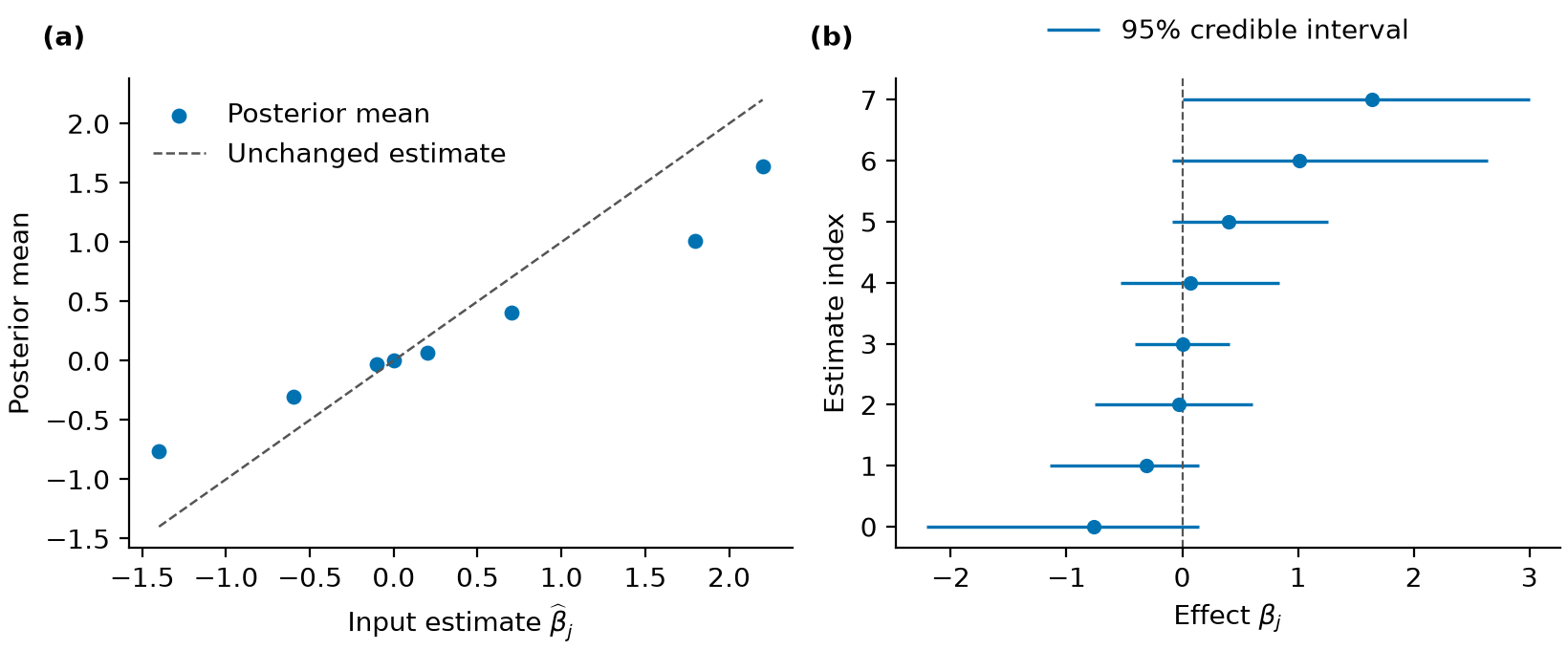
The two input vectors contain estimates and their standard errors. The normal-prior component standard deviations are fixed at the supplied scales; their weights are estimated. The first three posterior means are [-0.764278, -0.306851, -0.032956].

Student-t and asymmetric priors

student = fit(
    [-1.4, -0.6, -0.1], [0.7, 0.4, 0.5],
    family="uniform", scales=[0.5, 2.0], df=8,
)
asymmetric = fit(
    [-1.4, -0.6, -0.1, 0.0, 0.2, 0.7, 1.8, 2.2],
    [0.7, 0.4, 0.5, 0.3, 0.5, 0.4, 0.8, 0.7],
    family="halfuniform", scales=[0.5, 2.0],
)

A finite df selects the Student-t likelihood. Its second vector gives scale parameters, which are not Student-t standard deviations. halfuniform fits separate negative and positive uniform components. Inspect sign probabilities carefully; the prior grid and null-weight penalty affect their interpretation.

Poisson rates and binomial probabilities

from ashrink import fit_poisson, fit_binomial

rates = fit_poisson(
    [0, 1, 3, 8, 12], exposure=[1.0, 1.0, 2.0, 2.0, 3.0]
)
probabilities = fit_binomial([0, 2, 5, 8, 10], trials=10)
print(rates.summary())
print(probabilities.interval())

The Poisson posterior describes rates per exposure unit. The binomial posterior describes success probabilities. Both use conjugate mixtures sharing the specified mode. Their sign probabilities compare the parameter with null_value, rather than zero by default.

Effects across conditions

import numpy as np
from ashrink import fit_multivariate

effects = np.array([-1.4, -0.6, -0.1, 0.0])
paired = np.column_stack([effects, effects * 0.7])
multivariate = fit_multivariate(
    paired, np.full_like(paired, 0.5),
    covariances=[np.eye(2), np.ones((2, 2))],
    scales=[0.5, 1.5],
)
print(multivariate.format_summary())

Rows identify effects and columns identify conditions. The supplied covariance patterns describe independent effects and effects shared across both conditions. The fit estimates their mixture weights. It does not learn new covariance patterns.

Binary, count and grouped regression

from ashrink import (
    fit_logistic_regression, fit_poisson_regression,
    fit_mixed_regression,
)

X = np.array([[-1.0], [-0.5], [0.0], [0.5], [1.0], [1.5]])
binary = fit_logistic_regression(
    X, [0, 0, 1, 0, 1, 1], scales=[0.5, 1.0]
)
counts = fit_poisson_regression(
    X, [0, 1, 1, 2, 3, 4], exposure=1, scales=[0.5, 1.0]
)
grouped = fit_mixed_regression(
    X, [-1.0, 0.2, 1.0, 0.0, 1.2, 2.0],
    ["a"] * 3 + ["b"] * 3, scales=[0.5, 1.0],
)
print(binary.format_summary())
print(counts.format_summary())
print(grouped.random_effect_summary())

Logistic coefficients are on the log-odds scale; Poisson coefficients are on the log-rate scale. The grouped Gaussian model adds a random intercept for each group. These fixed examples demonstrate calls, not prediction accuracy or calibration.

Posterior summaries and data handling

Select a prior and likelihood

In fit, family selects the prior: normal, uniform or halfuniform. A finite df selects a Student-t likelihood; its input standard-error value is the distribution's scale, not its standard deviation. Gaussian inputs use the usual standard error. null_weight=1 fits mixture weights by maximum likelihood; larger values add a penalty favouring the point-null component.

normal_mixture and uniform_mixture construct explicit scalar priors. Pass one through fit(..., prior=prior, fix_prior=True) to evaluate a fixed prior without estimating new weights. Summary-input results provide shrink to evaluate new observations with the fitted prior, without estimating new weights. Student-t results require the new observations' df. For count results, shrink(observations, auxiliary) takes exposure times or trial counts as its second argument.

When observations are counts, shrinkage must respect the parameter range. Poisson rates are nonnegative and binomial probabilities lie between zero and one. The Poisson and binomial methods therefore use Gamma and Beta mixtures with a specified common mode. Their parameter and null scales differ from scalar signed effects. These are conjugate-mixture extensions, not matched R ashr likelihoods.

When effects are measured across conditions, their relationships can inform shrinkage. Multivariate fitting uses supplied positive-semidefinite covariance patterns and positive-definite observation-error covariances; patterns and residual correlations are not learned from the effects.

For regression inputs, see Regression models. Its coefficient distributions use a variational approximation; prediction returns outcome means.

Inspect posterior results

All results provide posterior_mean, posterior_sd, summary, cdf, quantile, interval and sample. summary returns reporting columns. Scalar, multivariate and regression results also have format_summary for compact text. sample draws latent parameters, not future observed data.

interval(level=.95) returns equal-tailed posterior credible intervals. They condition on the fitted mixture weights and selected component grid. lfdr is posterior point-null probability. lfsr is the smaller posterior probability of a nonpositive or nonnegative effect, including a zero atom in both error events. For count models, the directions are relative to the specified null rate or probability. qvalue and svalue average local null and sign-error probabilities at their respective cutoffs. They are posterior summaries, not automatic frequentist error-control guarantees. If the prior has no atom at the reported parameter's null value, lfdr and qvalue are zero by construction. This is a prior choice, not evidence against the null. In a multivariate model, a coordinate can retain an atom even without a whole-vector null component.

Multivariate results also provide posterior covariance matrices and the probability that the whole effect vector is zero. A coordinate can have a zero atom even when another coordinate does not. Marginal and whole-vector null probabilities therefore have different meanings.

Tables and saved results

Named-column adapters are fit_frame, fit_poisson_frame, fit_binomial_frame, fit_multivariate_frame and the regression _frame adapters. They accept pandas frames or mappings of columns. Scalar missing values are rejected by default; missing="drop" explicitly removes incomplete rows and retains their indices. Other fitting methods require complete data.

to_records returns plain rows; write_csv exports summaries. save_result and load_result use versioned JSON without pickle or code execution. Summary-input results reconstruct their posterior calculations; regression results restore their saved factors. Neither operation estimates new mixture weights. Saved results retain input estimates or counts. Regression JSON also retains training outcomes, directly or through fitted values and residuals; it is not an anonymized summary. result.to_dataframe() requires the table extra.

Plots

For summary-input fits, plot_shrinkage, plot_intervals, plot_prior and plot_diagnostics return Matplotlib axes. They do not call show or save files. For multivariate results, condition selects the column to display. Prior density plots keep point-null probability separate from continuous density. Regression has plot_coefficients and plot_residuals; plot_diagnostics displays the variational objective. Random-intercept fits also have plot_random_effects.

Regression models

Use fit_regression when the observations and predictors are available directly. Conditional on the fitted intercept and predictor transformation, coefficient fitting uses the Gaussian likelihood and prior

Here, \(n\) is the number of observations, \(p\) the number of predictors, and \(I_n\) the identity matrix. The \(K\) mixture weights satisfy \(\pi_k\ge0\) and \(\sum_k\pi_k=1\). The vector \(\mathbf y\) contains centered outcomes and \(\mathbf X\) contains centered, optionally scaled predictor columns. The vector \(\mathbf b\) contains coefficients on that predictor scale, and \(\sigma^2\) is the residual variance. With fit_intercept=False, outcomes and predictors are not centered. The regression prior \(g\) has mixture weights \(\pi_k\), which describe how often each prior scale occurs. A component with \(\sigma_k=0\) is a point mass at zero. The method follows Kim et al. (2024), Sections 3.1-3.5 and Appendix E.

Fit and predict

import numpy as np
from ashrink import fit_regression

X = np.array([[-1., -1.], [-1., 1.], [1., -1.], [1., 1.]])
y = np.array([-1.8, -0.1, 0.6, 3.3])
result = fit_regression(X, y, scales=[0.3, 1.0], labels=["x1", "x2"])
print(result.format_summary())
predicted = result.predict(np.array([[0.2, 0.5], [0.8, -0.3]]))

scales supplies the relative prior standard deviations \(\sigma_k\). Fitting adds a zero atom by default and learns the mixture weights and residual variance. The component grid is sorted and deduplicated; initial_weights must follow the resulting order, with the zero atom first.

The default fit includes an intercept and divides centered predictor columns by their root mean square. Returned coefficients and their intervals use the original predictor units. predict accepts numeric columns in the fitted order and reuses the fitted transformation. It returns outcome means, without prediction intervals. More predictors than observations are allowed; missing values and predictors with no information are rejected.

For named columns, use fit_regression_frame(data, outcome, predictors). For an aligned numerical comparison, disable standardization or reproduce its transformation explicitly. Fixed mixture weights and residual variance are available through estimate_weights=False and estimate_residual_variance=False, with their respective initial_* values.

Coefficients and diagnostics

coefficients, intercept, residual_variance and weights report fitted quantities. interval, cdf, quantile and sample describe approximate marginal coefficient distributions. summary returns numeric columns; plot_coefficients, plot_residuals and plot_diagnostics inspect the fit. Saved JSON includes fitted values and residuals, from which training outcomes can be recovered. It is not an anonymized summary.

The algorithm uses independent coefficient factors and maximizes an evidence lower bound (ELBO). Inspect diagnostics["converged"] and the recorded ELBO history. Convergence is local and can depend on initialization. The default starts coefficients at zero; initial_coefficients supplies another start.

Intervals condition on fitted mixture weights, residual variance and intercept. They do not include uncertainty from estimating those quantities. With strongly correlated predictors, the approximation can favor one predictor over another and understate uncertainty. Null/sign probabilities do not provide guaranteed variable selection or establish causal effects. The Gaussian method requires a dense numeric predictor matrix. Binary, count and grouped outcomes use the separate methods below.

Binary and count outcomes

Outcome	Function	Prediction
Binary outcomes or successes/trials	fit_logistic_regression(X, y, trials=1)	Probability; supply new trials for expected successes
Counts with exposure times	fit_poisson_regression(X, y, exposure=1)	Expected counts at new exposure

Both functions accept a numeric offset on the link scale. New predictions use exposure one and offset zero unless specified. Training row values are never reused for new rows. predict(..., scale="link") returns the linear predictor. Predictions apply the inverse link to mean coefficients; they do not integrate coefficient uncertainty. Poisson exponential underflow and overflow raise an error; link predictions can still represent extreme values.

Unlike Gaussian regression, these priors use absolute coefficient standard deviations on the transformed predictor scale. No residual variance is fitted. Logistic coefficients describe log odds; Poisson coefficients describe log rates. Their intervals remain approximate marginal credible intervals.

Logistic fitting uses the quadratic lower bound of Jaakkola and Jordan (1997). Poisson fitting evaluates its expected log likelihood using the exponential moments of the mixture-normal factors. It then optimizes component means and variances with safeguarded Newton steps. Both methods estimate mixture weights and report their variational objective. These are extensions beyond the scalar ASH likelihoods, rather than matched R ashr methods.

Grouped continuous outcomes

fit_mixed_regression(X, y, groups) adds independent Gaussian random intercepts to Gaussian regression. Supply one nonempty string group label per observation. The fit estimates a common group variance as well as the residual variance. The estimate_group_variance and estimate_residual_variance flags can hold supplied initial values fixed.

result.predict(X_new) returns population means. Supplying known group labels adds their fitted random intercepts. Unseen labels raise an error unless allow_new_groups=True, which assigns those groups a mean random effect of zero. Neither choice adds future observation noise or integrates uncertainty in the group effects.

random_effect_summary and random_effect_interval report the approximate group distributions; plot_random_effects displays them. Fixed and group factors are independent in the variational approximation. Their marginal variances need not equal those from an exact joint Gaussian analysis. Random slopes, general correlation structures and non-Gaussian mixed models are outside this version.

The worked examples show all three methods. Named-column adapters add _frame to each fitting function's name. fit_mixed_regression_frame takes the group column through group=.

Numerical methods and interpretation

The scalar implementation estimates finite-mixture weights for the adaptive-shrinkage models described by Stephens (2017). Gaussian component posteriors are analytic. Student-t component posteriors use adaptive one-dimensional quadrature and record integration diagnostics. Quadrature can be substantially slower than the analytic Gaussian calculation.

Mixture fitting uses expectation-maximization (EM) with fixed component grids, followed by constrained optimization when the optimality residual remains large. Diagnostics retain the objective history, iteration count, stopping rule and a Karush-Kuhn-Tucker (KKT) optimality residual. A small residual is a numerical stopping criterion; it does not establish statistical calibration or uniqueness of the fitted prior. Results retain nonconvergence information rather than treating every returned fit as reliable.

The R reference version is ashr 2.2-63. Uniform widths and normal standard deviations have different meanings. Student-t inputs are scale parameters. The normal-prior/Student-t combination uses an independent integration method; the inspected R implementation rejects that combination. Ranked summaries include all tied local probabilities at a cutoff, which can differ from R's order-dependent cumulative averages within ties.

Count models use conjugate Gamma-Poisson and Beta-binomial mixtures sharing a specified mode, with an optional point mass at that mode. Multivariate models use finite mixtures of zero-mean normals with supplied covariance patterns, following the fixed-pattern part of Urbut et al. (2019). AShrink does not implement all methods in ashr or mashr.

Posterior probabilities and credible intervals condition on estimated mixture weights. They omit uncertainty from fitting those weights. Dependence between scalar observations, misspecified likelihoods and unsuitable prior components can affect inference. The numerical reference checks below describe the comparisons and their limits.

Gaussian regression uses cyclic variational coordinate ascent with residual-variance-scaled normal-mixture priors, following Kim et al. (2024). The objective is an evidence lower bound, rather than the exact marginal likelihood. Coefficient marginals factorize; their variances need not equal those from the exact joint posterior. Mean predictions reuse fitted preprocessing. See Regression models for inputs and limits.

Binary/binomial regression uses a quadratic logistic lower bound. Poisson regression uses analytic exponential moments of independent mixture-normal factors, with guarded inner Newton optimization. Gaussian random-intercept regression uses independent coefficient and group factors. These extensions have focused analytic and stationarity checks, not repeated-dataset calibration studies. Prediction applies the fitted mean coefficients; nonlinear predictions do not integrate their uncertainty. See Regression models.

Numerical reference checks

The test fixtures contain six scalar cases from installed R ashr 2.2-63 and five Gaussian regression cases from installed mr.ash.alpha 0.1-43 (commit 8e257fdb73589f280192b1c99a176d82196be298). Three multivariate cases also use installed mashr 0.2.79. All exports used R 4.5.1. Archive and exporter hashes are stored with each fixture.

Comparison	Quantities	Absolute and relative tolerance
Gaussian scalar, fixed prior	Mean, SD, null/sign probabilities, weights	2e-11
Student-t/uniform scalar, fixed prior	Same quantities	2e-7
Gaussian scalar, estimated weights	Same quantities	2e-6
Gaussian regression, converged fit	Coefficients, intercept, residual variance, weights	1e-5
Gaussian regression, one sweep	Same quantities	2e-10
Multivariate, fixed prior or one component	Means, SDs, covariance, null/sign probabilities, weights	2e-10
Multivariate, estimated mixture	Same quantities	5e-6

Regression comparisons use explicit grids, zero initial coefficients, common initial weights/variance, an intercept and no standardization. R uses method_q="sigma_indep_q", matching the fixed-factor variance update. Its sigma_dep_q option uses a different update and need not agree after one sweep. Stopping rules also differ: AShrink checks changes in the evidence lower bound (ELBO), whereas R checks coefficient or mixture-weight changes. Matching results in these cases does not establish global optimization, interval coverage or prediction performance.

R warns that half-uniform priors without a null-biased penalty can give misleading sign probabilities. Those fixed-prior cases check arithmetic only. The regression reference also warns when substantial weight reaches the largest prior component. The comparison keeps the explicit grid unchanged; an applied analysis should inspect its adequacy.

Conjugate count models and fixed-pattern multivariate models have independent analytic tests. Their inclusion does not imply full ashr or mashr coverage. Logistic and Poisson-regression tests check null-only likelihoods and the stationarity equations for a single normal factor. Random-intercept tests compare fixed-variance posterior means with a joint Gaussian block solution. These checks address the implemented updates; they do not establish interval coverage or prediction performance across repeated datasets.

Multivariate comparisons use explicit covariance patterns, correlation matrices, unit scale multipliers and no automatic covariance normalization. One case checks a single full-rank component, one estimates mixture weights, and one reconstructs fixed-weight summaries with singular patterns and a zero atom. The fixed-weight case uses mash(..., fixg=TRUE) in R and public result reconstruction in Python. It checks posterior calculations rather than fitting new mixture weights. R's one-component optimizer reports that no optimization is needed. Learning covariance patterns is not supported.

Function reference

Required arguments have no default in the signatures below. Arguments with a default can be omitted. An input may still be required by another choice; for example, an explicit covariance matrix is an alternative to standard errors in multivariate fitting. All names below are imported from ashrink.

Scalar and count models

fit

fit(
    effects,
    standard_errors,
    *,
    family='normal',
    df=None,
    scales=None,
    point_mass=True,
    null_weight=1,
    prior=None,
    fix_prior=False,
    maxiter=10000,
    tol=1e-08,
    missing='raise',
    labels=None,
)

Fit a zero-mode scalar mixture prior and obtain posterior summaries.

family chooses the prior: normal, uniform, or halfuniform. Errors are Gaussian unless positive finite df requests a Student-t likelihood; standard_errors is then the Student-t scale, not its standard deviation. Infinite df selects Gaussian errors. Finite and infinite df may be mixed. Supplied scales are normal SDs or uniform half-widths. The default grid follows ashr 2.2-63's geometric rule, with spacing sqrt(2).

null_weight >= 1 adds (null_weight - 1) log(pi0) to the objective. A supplied prior supplies the grid and starting weights; fix_prior=True also fixes those weights. Missing rows are rejected unless missing='drop'. Neither intervals nor local error probabilities account for uncertainty in estimated mixture weights. Student-t quadrature is slower than the analytic Gaussian path; inspect diagnostics for integration accuracy.

normal_mixture

normal_mixture(scales, weights=None, point_mass=True)

Construct zero-mean normal components, optionally with a zero atom.

scales contains standard deviations. Duplicates are removed and the resulting grid is sorted. Supplied weights refer to that final grid, including its leading zero atom when requested.

uniform_mixture

uniform_mixture(widths, weights=None, asymmetric=False, point_mass=True)

Construct symmetric or separate left/right uniform components.

Positive widths a produce [-a,a], or [-a,0] followed by [0,a] when asymmetric=True. Within each side widths are sorted. A requested zero atom comes first; supplied weights refer to this final component order.

fit_poisson

fit_poisson(
    counts,
    exposure=1,
    *,
    null_value=1,
    strengths=None,
    point_mass=True,
    null_weight=1,
    maxiter=10000,
    tol=1e-08,
)

Shrink Poisson rates under a fitted mode-shared gamma mixture.

Counts follow a Poisson distribution with mean exposure[i] * rate[i]. Continuous Gamma components have shape 1 + null_value * strength and rate strength. The default grid is 2**arange(-4, 9). null_weight-1 is a nonnegative null-atom pseudo-count, not an observation weight. No missing values are accepted.

fit_binomial

fit_binomial(
    successes,
    trials,
    *,
    null_value=0.5,
    strengths=None,
    point_mass=True,
    null_weight=1,
    maxiter=10000,
    tol=1e-08,
)

Shrink binomial probabilities under a fitted mode-shared beta mixture.

Beta components have parameters 1 + null_value * strength and 1 + (1 - null_value) * strength. The default grid is 2**arange(-4, 9). Trials may be scalar; zero trials are allowed only with zero successes and contribute no likelihood evidence. null_weight-1 penalizes the null atom as a nonnegative pseudo-count.

Multivariate models

fit_multivariate

fit_multivariate(
    effects,
    standard_errors=None,
    *,
    error_covariance=None,
    correlation=None,
    covariances=None,
    scales=None,
    point_mass=True,
    null_weight=1,
    maxiter=10000,
    tol=1e-08,
)

Fit a finite mixture of fixed multivariate normal covariance patterns.

Parameters

• effects (array, shape (n,d)). Finite effect estimates; d must be at least two. Rows are independent.

• standard_errors (array, shape (n,d)). Positive standard errors. Used with a supplied residual correlation matrix or the identity. Alternatively supply error_covariance.

• error_covariance (array, shape (d,d) or (n,d,d)). Positive definite observation-error covariance. Cannot be combined with standard errors or a correlation matrix.

• correlation (array, shape (d,d)). Positive definite residual correlation, treated as known.

• covariances (array, shape (k,d,d)). Positive semidefinite prior patterns; singular patterns are allowed. Defaults to identity, equal-effect and single-condition patterns.

• scales (nonnegative vector). Standard-deviation multipliers: components are scale**2 times each pattern. With supplied patterns the default is [1]. Canonical patterns use [0.1,0.25,0.5,1,2,4] times the median standard error.

• point_mass (bool). Include one all-zero component. Zero components supplied through the grid are retained even when False; duplicates are removed exactly.

• null_weight (float >= 1). Dirichlet parameter for the joint null; 1 gives maximum likelihood. A value above one requires a joint-null component.

• maxiter, tol (int, float). Total EM/SLSQP iteration limit and weight-change warmup tolerance. Final convergence uses the relative KKT residual with threshold max(1e-7, 10*tol); inspect diagnostics.

Notes

Mixture weights are estimated on all supplied rows. Do not select only significant rows before learning the prior. Posterior summaries condition on the fitted weights, patterns and error covariance. No covariance-pattern learning or missing-condition imputation is performed. PSD eigenvalues at most 1e-12 times their largest absolute eigenvalue are treated as roundoff.

Regression models

fit_regression

fit_regression(
    X,
    y,
    *,
    scales=None,
    point_mass=True,
    fit_intercept=True,
    standardize=True,
    estimate_weights=True,
    estimate_residual_variance=True,
    initial_coefficients=None,
    initial_weights=None,
    initial_residual_variance=None,
    maxiter=1000,
    tol=1e-06,
    labels=None,
)

Fit Gaussian multiple regression with a normal-mixture shrinkage prior.

For transformed predictors, y = X b + error with error variance sigma^2, and b_j has prior sum_k pi_k N(0, sigma^2 * scales[k]^2). A scale of zero denotes a point mass at zero. Supplied scales are standard deviations relative to the residual SD, not component variances. The default uses scales 2**(0.05*k)-1 for k=0,...,19, following mr.ash's 20-point grid. Duplicate scales are removed and the grid is sorted. Initial weights refer to this final order, including the leading zero atom when requested.

X is a finite dense (n,p) array and y has length n. Standardization divides each centered column by its root mean square (divisor n). With no intercept, columns and y are not centered. Coefficients, intervals and initial_coefficients use original predictor units. Columns with zero information after centering are rejected; the intercept is fitted separately.

Each sweep updates coefficient factors, then mixture weights and residual variance while holding those factors fixed (Kim et al., 2024, Appendix E). Set either estimate_* flag to False to retain its initial value. The residual-variance update divides its expected quadratic terms by n plus the sum of posterior probabilities of nonzero coefficients. This is the fixed-factor update of Kim et al. (2024), Appendix E.3. ELBO convergence is a local stopping criterion, not evidence of a global optimum or calibrated variable selection.

fit_logistic_regression

fit_logistic_regression(
    X,
    y,
    *,
    trials=1,
    offset=0,
    scales=None,
    point_mass=True,
    fit_intercept=True,
    standardize=True,
    estimate_weights=True,
    initial_coefficients=None,
    initial_weights=None,
    initial_intercept=None,
    maxiter=1000,
    tol=1e-06,
    labels=None,
)

Fit binomial logistic regression with adaptive normal-mixture priors.

y contains successes and trials contains totals; binary outcomes use trials one. The prior scales are absolute coefficient SDs after predictor transformation, with no Gaussian residual-variance factor. Scales are sorted and deduplicated; initial weights refer to that final grid, including a leading zero atom when requested. Defaults are 0.25, 0.5, 1, 2 and 4. Initial coefficients use original predictor units; initial_intercept is the intercept for the transformed design. Returned intercepts use original units.

Zero-trial rows remain in the result but do not determine predictor centering or scaling. Inputs are finite dense arrays; missing values are rejected. An unpenalized intercept requires at least one success and one failure. Fitting maximizes a Jaakkola--Jordan lower bound using independent coefficient factors. Its intervals are approximate marginal credible intervals, conditional on fitted weights and intercept.

fit_poisson_regression

fit_poisson_regression(
    X,
    y,
    *,
    exposure=1,
    offset=0,
    scales=None,
    point_mass=True,
    fit_intercept=True,
    standardize=True,
    estimate_weights=True,
    initial_coefficients=None,
    initial_weights=None,
    initial_intercept=None,
    maxiter=1000,
    tol=1e-06,
    inner_maxiter=100,
    inner_tol=1e-08,
    labels=None,
)

Fit Poisson log-link regression with adaptive normal-mixture priors.

Expected counts are exposure * exp(intercept + offset + X b). Exposures must be positive. Prior scales are absolute SDs on transformed coefficients; no Gaussian residual variance is fitted. Scales are sorted and deduplicated, and initial weights use that order with a leading zero atom when requested. Initial coefficients use original predictor units; initial_intercept is the intercept for the transformed design. Returned intercepts use original units.

The algorithm uses the exact expected Poisson log likelihood within the independent mixture-normal approximation. Positive-component means and variances are optimized by damped Newton steps. Failed inner optimization and nonfinite exponential moments raise an error. Coefficient intervals remain approximate, conditional on fitted weights and intercept.

fit_mixed_regression

fit_mixed_regression(
    X,
    y,
    groups,
    *,
    scales=None,
    point_mass=True,
    fit_intercept=True,
    standardize=True,
    estimate_weights=True,
    estimate_residual_variance=True,
    estimate_group_variance=True,
    initial_weights=None,
    initial_residual_variance=None,
    initial_group_variance=None,
    initial_coefficients=None,
    maxiter=1000,
    tol=1e-06,
    labels=None,
)

Fit Gaussian regression with shrunk coefficients and random intercepts.

y_i = alpha + x_i b + u_groups[i] + error_i, with independent u_g ~ N(0,tau^2) and errors ~ N(0,sigma^2). On transformed predictors, b_j follows sum_k pi_k N(0,sigma^2*scales[k]^2), including a zero atom when requested. Group labels must be nonempty strings; convert numeric identifiers to strings before fitting. No random slopes or GLMM is fitted.

Coordinate ascent uses independent coefficient and group variational factors. Each estimate_* flag can fix its supplied starting parameter. The intercept is unpenalized; centering and RMS scaling match fit_regression. The default grid is 2**(0.05*k)-1 for k=0,...,19. Initial coefficients and returned coefficient summaries use original predictor units.

Named-column inputs

fit_frame

fit_frame(
    data,
    estimate='estimate',
    standard_error='se',
    *,
    label=None,
    df=None,
    **options,
)

Fit scalar effects from a pandas DataFrame or mapping of columns.

df may name a column of Student-t degrees of freedom or supply numeric degrees of freedom. A label column is retained for result tables.

fit_poisson_frame

fit_poisson_frame(data, count='count', exposure='exposure', **options)

Fit Poisson rates from named count and exposure columns.

fit_binomial_frame

fit_binomial_frame(data, successes='successes', trials='trials', **options)

Fit binomial probabilities from named success and trial columns.

fit_multivariate_frame

fit_multivariate_frame(data, estimates, standard_errors, **options)

Fit effect/SE matrices assembled from matching named columns.

fit_regression_frame

fit_regression_frame(data, outcome, predictors, **options)

Fit Gaussian regression from an outcome and named numeric predictors.

fit_logistic_regression_frame

fit_logistic_regression_frame(
    data,
    outcome,
    predictors,
    *,
    trials=1,
    offset=0,
    **options,
)

Fit logistic regression; trials and offset may name numeric columns.

fit_poisson_regression_frame

fit_poisson_regression_frame(
    data,
    outcome,
    predictors,
    *,
    exposure=1,
    offset=0,
    **options,
)

Fit Poisson regression; exposure and offset may name numeric columns.

fit_mixed_regression_frame

fit_mixed_regression_frame(data, outcome, predictors, *, group, **options)

Fit Gaussian random intercepts from a named string group column.

Tables and saved results

read_csv

read_csv(path)

Read a headered numeric CSV into a mapping of NumPy columns.

to_records

to_records(result, *, level=0.95)

Return one plain record per observation and condition.

Bounds are equal-tailed empirical-Bayes posterior credible intervals, conditional on the fitted mixture weights.

write_csv

write_csv(result, path, *, level=0.95, overwrite=False)

Write posterior summaries to a headered CSV file.

save_result

save_result(result, path, *, overwrite=False)

Save a versioned JSON result; no executable objects are stored.

A new file is required unless overwrite=True. Serialization finishes before the destination is opened.

load_result

load_result(path)

Restore posterior calculations from a JSON result without refitting.

Plots

plot_shrinkage

plot_shrinkage(result, *, condition=0, ax=None)

Compare input estimates with posterior means on the same scale.

Binomial rows with zero trials have no observed proportion and are omitted from this display; they remain in the fitted result.

plot_intervals

plot_intervals(result, *, condition=0, level=0.95, indices=None, ax=None)

Show equal-tailed posterior credible intervals and posterior means.

Each horizontal line represents a retained observation. The interval conditions on fitted mixture weights; it is not a frequentist confidence interval or an interval for a future observation.

plot_prior

plot_prior(result, values=None, *, condition=0, ax=None)

Display continuous prior density; show point-null mass separately.

An atom is a probability, not a density height. Its mass is labelled in the legend rather than drawn as an infinite density spike.

plot_diagnostics

plot_diagnostics(result, *, ax=None)

Display the recorded optimization objective by optimization iteration.

plot_coefficients

plot_coefficients(result, *, level=0.95, indices=None, ax=None)

Show approximate marginal regression intervals on the coefficient scale.

These variational intervals condition on fitted hyperparameters; they do not include uncertainty in the intercept or residual variance.

plot_residuals

plot_residuals(result, *, ax=None)

Plot observed residuals against fitted response means.

plot_random_effects

plot_random_effects(result, *, level=0.95, ax=None)

Display approximate Gaussian random-intercept marginal intervals.

Result classes

Obtain results from fitting functions or load_result; constructing the internal posterior arrays directly is unnecessary for an analysis. The shared methods below operate on latent parameters. They do not generate future outcomes.

Method	Meaning
cdf(value)	Posterior probability at or below value
quantile(probability)	Marginal posterior quantile; probabilities lie in [0, 1]
interval(level=0.95)	Equal-tailed marginal credible interval
sample(size=1, seed=None)	Reproducible draws of latent effects or coefficients
summary(level=0.95)	Numeric reporting columns
to_dataframe(level=0.95)	pandas table; requires the table extra
to_dict() / from_dict(value)	Portable result representation and reconstruction

MixturePrior

A fixed component grid and its mixture probabilities.

Use normal_mixture or uniform_mixture to construct a grid. All components have mode zero; asymmetric uniform components may have different weights on either side of zero.

with_weights(weights)

Return a prior with the same components and the supplied normalized weights.

density(x)

Continuous density only; null_mass gives the zero atom.

cdf(x)

Right-continuous CDF, including the zero atom.

to_dict()

from_dict(value)

to_json()

from_json(text)

ASHResult

Scalar mixture posterior summaries conditional on a fitted prior.

lfdr is the posterior zero-atom probability. lfsr is the smaller posterior probability of a nonpositive or nonnegative effect, so the atom belongs to both error events. Strict negative/positive probabilities exclude it. Credible intervals condition on estimated weights, not uncertainty in those weights. Missing rows are absent and row_indices maps back to the original input. Public numeric arrays are read-only.

prior_density(x)

prior_cdf(x)

cdf(value)

Posterior probability of an effect at or below value; supply one threshold or one threshold per row.

quantile(probability)

Quantiles: scalar -> (n,), levels vector -> (levels, n).

interval(level=0.95)

Equal-tailed posterior interval, conditional on the fitted prior.

sample(size=1, seed=None)

Draw (size, n) posterior samples, conditional on the fitted prior.

summary(level=0.95)

Numeric reporting columns, without a pandas dependency.

format_summary(level=0.95, digits=6)

A compact text summary with at most twelve rows.

to_dataframe(level=0.95)

Return summary columns; requires the optional pandas dependency.

shrink(effects, standard_errors, df=None, *, missing='raise', labels=None)

Apply the fitted prior to new observations without estimating weights.

Student-t fits require degrees of freedom for the new observations; degrees of freedom attached to old rows are not silently reused.

to_dict()

JSON-compatible inputs, fitted prior and diagnostics (schema 1).

from_dict(value)

Rebuild component posteriors from stored inputs without fitting weights.

save(path)

Save a versioned JSON result, without pickle or executable objects.

load(path)

CountResult

Fitted conjugate mixture and marginal posterior summaries.

probability_below_null and probability_above_null are strict tail probabilities. lfsr includes equality in both directional error events. qvalue averages null probabilities at each tied null-probability cutoff; svalue does the same for lfsr. These are posterior summaries, not claims of frequentist error control.

shrink(observations, auxiliary=1)

Evaluate new observations using the fitted prior without refitting.

auxiliary gives exposure for a Poisson result or trials for a binomial result. It may be scalar or one value per observation. Supply the appropriate new exposure times or trial counts explicitly when they differ from one. The original grid, null and mixture weights are reused; the original observations are not added to the new likelihood.

cdf(value)

Return the posterior probability of a rate or probability at or below value; supply one threshold or one threshold per row.

quantile(prob)

Posterior generalized inverse CDF; levels by observations for 1D input.

interval(level=0.95)

Equal-tail posterior credible intervals, one row per observation.

sample(size=1, seed=None)

Draw posterior samples; result shape is (size, observations).

prior_density(value)

Continuous prior density; the null atom is excluded.

prior_cdf(value)

Prior CDF, including the null atom.

summary(level=0.95)

Return numeric columns for reporting; no pandas dependency.

to_dataframe(level=0.95)

Return summary columns as a pandas DataFrame (requires pandas).

to_dict()

from_dict(data)

Restore a stored mixture without optimizing weights again.

save(path)

load(path)

MultivariateResult

Posterior summaries for fixed-pattern multivariate shrinkage.

lfdr is the marginal probability of an exactly zero effect, which may include condition-specific atoms. joint_null_probability refers only to the component whose whole effect vector is zero. Fitted-prior summaries do not integrate uncertainty in the estimated mixture proportions.

cdf(value)

Marginal posterior probability at or below value, including zero atoms.

prior_density(value, *, condition=0)

Continuous marginal fitted-prior density, excluding zero atoms.

value can have any shape. condition selects a matrix column. The excluded probability is prior_null_probability[condition].

prior_cdf(value, *, condition=0)

Marginal fitted-prior CDF for one condition, including zero atoms.

shrink(new_effects, standard_errors=None, *, error_covariance=None, correlation=None)

Evaluate new independent rows using the exact fitted prior.

New rows do not update covariance patterns or mixture weights. Supply their standard errors or error covariances explicitly.

quantile(probability)

Marginal generalized-inverse CDF, not a simultaneous region.

A scalar returns (n,d); a one-dimensional probability vector returns (levels,n,d). Endpoints are infinite for unbounded marginals.

interval(level=0.95)

Equal-tailed marginal credible intervals, with shape (n,d,2).

sample(size=1, seed=None)

Draw conditional posterior samples with shape (size,n,d).

summary(level=0.95)

Return numeric (n,d) reporting columns without requiring pandas.

format_summary()

Return a short human-readable description of the result.

to_dataframe(level=0.95)

Return a long table; install the separate table extra for pandas.

to_dict()

Return JSON-compatible inputs and fitted weights; no executable data.

from_dict(value)

Reconstruct summaries with fixed weights, without optimization.

RegressionResult

Variational coefficient distributions for Gaussian regression.

Coefficients and their component distributions use the original predictor units. scales instead describes the prior on the transformed design: component k has variance residual_variance * scales[k]**2. Intercept estimation and hyperparameter uncertainty are not included in the marginal coefficient intervals. Correlated predictors can have underestimated joint uncertainty under the factorized approximation.

predict(X)

Predict the outcome mean for a finite (n_new,p) numeric matrix.

The fitted centering and scaling are already incorporated in the original-unit coefficients and intercept. No prediction interval or extra observation noise is included.

cdf(value)

Approximate marginal coefficient probability at or below value, including zero atoms.

quantile(probability)

Approximate marginal quantiles; scalar gives (p,), vector gives (levels,p).

interval(level=0.95)

Equal-tailed approximate marginal credible intervals, shape (p,2).

sample(size=1, seed=None)

Draw (size,p) coefficients independently from variational factors.

summary(level=0.95)

Return coefficient reporting columns; all uncertainty is approximate.

format_summary(level=0.95, digits=4)

Return a compact coefficient table and the optimizer status.

to_dataframe(level=0.95)

Return coefficient summaries; requires the separate table extra.

to_dict()

Return versioned variational factors and prediction transformations.

Training fitted values and residuals are included. Saving this result therefore retains information about training outcomes.

from_dict(document)

Restore saved factors without fitting or recomputing the posterior.

save(path, *, overwrite=False)

Save JSON using the shared persistence interface.

load(path)

Load a Gaussian regression result using the shared JSON reader.

GLMResult

Approximate coefficients and plug-in predictions for a fitted GLM.

Logistic coefficients are log odds per predictor unit; Poisson coefficients are log rates per predictor unit. Coefficient intervals condition on fitted mixture weights and the estimated intercept. They exclude hyperparameter and intercept uncertainty. Predictions apply the inverse link to the mean coefficients; they do not integrate the coefficient distributions.

cdf(value)

quantile(probability)

interval(level=0.95)

Approximate marginal coefficient credible intervals, shape (p,2).

sample(size=1, seed=None)

Independent variational coefficient draws, shape (size,p).

predict(X, *, scale='response', trials=None, exposure=1, offset=0)

Predict using mean coefficients and new-row offsets.

scale='link' returns log odds or log expected counts. On the response scale logistic output is a probability unless trials is supplied, when it is expected successes. Poisson output is expected counts at the supplied exposure. New rows default to exposure one and offset zero; training offsets are never reused.

summary(level=0.95)

Return approximate coefficient distributions on the link scale.

format_summary(level=0.95, digits=4)

to_dataframe(level=0.95)

Return coefficient summaries; requires the table extra.

to_dict()

Serialize factors and training responses without refitting.

from_dict(document)

save(path, *, overwrite=False)

load(path)

MixedRegressionResult

Fitted fixed-effect factors and Gaussian group-intercept factors.

Fixed-effect summaries and coefficient distribution methods follow RegressionResult; the methods below add group-specific outputs and predictions. Fixed effects use original predictor units. All intervals are approximate marginal credible intervals conditional on fitted hyperparameters. They exclude intercept uncertainty and covariance between coefficient factors. Group identifiers are case-sensitive nonempty strings.

predict(X, groups=None, *, allow_new_groups=False)

Predict population means, or conditional means for supplied groups.

With groups=None, no group effect is added. Unknown group labels raise unless allow_new_groups=True, which assigns their prior mean zero. Neither choice adds observation noise or supplies prediction intervals.

random_effect_interval(level=0.95)

Approximate marginal group-intercept intervals, shape (n_groups,2).

random_effect_summary(level=0.95)

random_effect_intervals(level=0.95)

Alias for random_effect_interval, with one interval per fitted group.

summary(level=0.95)

Return fixed-effect reporting columns; group summaries are separate.

format_summary(level=0.95, digits=4)

to_dict()

Serialize fitted factors, including training outcomes via residuals.

from_dict(document)

Restore stored factors without optimization or executable objects.

save(path, *, overwrite=False)

load(path)

References and attribution

• Stephens, M. (2017). False discovery rates: a new deal. Biostatistics, 18, 275-294. DOI.
• Urbut, S. M., Wang, G., Carbonetto, P., and Stephens, M. (2019). Flexible statistical methods for estimating and testing effects in genomic studies with multiple conditions. Nature Genetics, 51, 187-195. DOI.
• Kim, Y., Wang, W., Carbonetto, P., and Stephens, M. (2024). A flexible empirical Bayes approach to multiple linear regression and connections with penalized regression. Journal of Machine Learning Research, 25(185), 1-59. Article.
• Jaakkola, T. S., and Jordan, M. I. (1997). A variational approach to Bayesian logistic regression models and their extensions. Proceedings of the Sixth International Workshop on Artificial Intelligence and Statistics, 283-294. Article.

AShrink is an independent Python implementation. The R packages ashr, mashr and mr.ash.alpha provide matched numerical references where specified; their authors have not endorsed AShrink. See the repository's NOTICE and LICENSE for software attribution and license terms.